A Deep Learning Method for Bias Correction of ECMWF 24–240 h Forecasts

Lei HAN ,Mingxuan CHEN ,Kangkai CHEN ,Haonan CHEN ,Yanbiao ZHANG ,Bing LU ,Linye SONG,and Rui QIN

1College of Information Science and Engineering,Ocean University of China,Qingdao 266100,China

2Institute of Urban Meteorology,China Meteorological Administration,Beijing 100089,China

3Department of Electrical and Computer Engineering,Colorado State University,Fort Collins,CO 80523,USA

ABSTRACT Correcting the forecast bias of numerical weather prediction models is important for severe weather warnings.The refined grid forecast requires direct correction on gridded forecast products,as opposed to correcting forecast data only at individual weather stations.In this study,a deep learning method called CU-net is proposed to correct the gridded forecasts of four weather variables from the European Centre for Medium-Range Weather Forecast Integrated Forecasting System global model (ECMWF-IFS):2-m temperature,2-m relative humidity,10-m wind speed,and 10-m wind direction,with a forecast lead time of 24 h to 240 h in North China.First,the forecast correction problem is transformed into an image-toimage translation problem in deep learning under the CU-net architecture,which is based on convolutional neural networks.Second,the ECMWF-IFS forecasts and ECMWF reanalysis data (ERA5) from 2005 to 2018 are used as training,validation,and testing datasets.The predictors and labels (ground truth) of the model are created using the ECMWF-IFS and ERA5,respectively.Finally,the correction performance of CU-net is compared with a conventional method,anomaly numerical correction with observations (ANO).Results show that forecasts from CU-net have lower root mean square error,bias,mean absolute error,and higher correlation coefficient than those from ANO for all forecast lead times from 24 h to 240 h.CU-net improves upon the ECMWF-IFS forecast for all four weather variables in terms of the above evaluation metrics,whereas ANO improves upon ECMWF-IFS performance only for 2-m temperature and relative humidity.For the correction of the 10-m wind direction forecast,which is often difficult to achieve,CU-net also improves the correction performance.

Key words:numerical weather prediction,bias correction,deep learning,ECMWF

1.Introduction

Accurate weather forecasting can improve social and economic value in many areas such as transportation,aviation,agriculture,and water resources management.At present,operational weather forecasts depend mainly on numerical weather prediction (NWP) models,which have undergone significant improvement over the past four decades (

Bauer et al.,2015

;

Rasp and Lerch,2018

).Due to inevitable errors in representing atmospheric dynamics and physics,numerical models continue to introduce forecast bias (

Vashani et al.,2010

;

Peng et al.,2013

;

Xue et al.,2015

;

Vannitsem et al.,2020

).Developing post-processing methods to reduce forecast bias is essential to improving the forecasting skill of numerical models.Many model bias correction methods have been proposed over the past decades (

Houtekamer and Mitchell,

1998

;

Hu et al.,2014

;

He et al.,2019

;

Xia et al.,2020

).Therein,model output statistics (MOS) and perfect prog(PP) are two commonly used methods (

Marzban et al.,2006

).MOS mainly uses observation data to match the output of NWP and then obtains a prediction equation based on linear regression (

Glahn and Lowry,1972

).The PP method is similar to MOS,but it establishes a linear statistical relationship between observations and the NWP model analysis to accomplish the correction (

Klein et al.,1959

).These two methods provide a basis for enhancing prediction capability through their combination and introduction of new functionalities.For example,

Vislocky and Young (1989)

used PP forecasts as predictors in MOS to improve the accuracy of statistical precipitation probability models for forecasting.

Marzban (2003)

introduced an artificial neural network to replace the linear relationship in post-processing of surface observations for temperature predictions.The Kalman filter technique has also been applied for bias correction,to adjust the regression equation coefficients in real time,as opposed to MOS,which does not have this capability (

Homleid,1995

).

Cho et al.(2020)

used various machine learning methods,such as random forest and support vector machine,to establish statistical relationships between the predictor and predictand.However,almost all the above correction approaches focus on correcting forecast data at individual weather observation stations.Refined grid forecasting is becoming increasingly important in weather prediction models.Thus,the development of grid point-based forecast-bias correction techniques is an urgent challenge (

Vannitsem et al.,2020

).Using the theory of the decomposition of atmospheric variables presented by

Qian (2012)

,

Peng et al.(2013)

proposed the anomaly numerical correction with observations(ANO) method,in which both observations and numerical predictions can be decomposed into a climate mean and a perturbation value.The difference in the climate mean between model forecasts and real observations represents the systematic model bias (

Chang et al.,2015

).ANO can output gridded bias correction results by applying the modelled bias to each grid cell and is used in the current study as a benchmark to compare the correction performance of the proposed deep learning method.In recent years,deep learning techniques have achieved outstanding success in many fields,including atmospheric science (e.g.,

Rasp and Lerch,2018

;

Boukabara et al.,2019

;

Chen et al.,2019

).Deep learning can execute feature engineering on its own and automatically detect spatial structures in gridded data,which traditional ML cannot do.Another strength of deep learning is that it can create transferable solutions.Once a given deep-learning architecture is found to be successful for one problem,the same architecture may be successful for a similar problem.Also,a deep-learning model trained for one problem can often be "fine-tuned" (e.g.,weights in the last few layers can be retrained) for a different problem.In other words,not only the architecture,but also the learned weights,can be reused.This is often called"transfer learning".

Shi et al.(2015

,

2017)

first introduced a novel deep learning method,referred to as a convolutional long short-term memory (ConvLSTM) network,to improve precipitation nowcasting performance.

Guo et al.(2020)

used a gated recurrent unit to replace LSTM in an effort to reduce computational complexity.Relatively speaking,since it is easier to be transplanted to various problems,convolutional neural networks (CNN) methods are more often used in meteorological applications (e.g.,

Tao et al.,2016

;

Lagerquist et al.,2019

;

Lebedev et al.,2019

;

Han et al.,2020

).

Tao et al.(2016)

proposed a stacked denoising autoencoder network to reduce satellite precipitation estimation bias.

Lebedev et al.(2019)

used a CNN to reconstruct the satellite image for precipitation forecasts.

Han et al.(2020)

constructed a convolutional network with three-dimensional convolution to fuse multi-source data for convective storm nowcasting,which yielded better performance compared to traditional machine learning methods.

Lagerquist et al.(2019)

used a CNN to identify fronts in gridded data for spatially explicit prediction of synoptic-scale fronts.All the above deep learning methods improve on traditional methods.As a CNN-based network,U-net was proposed first in the image segmentation field;segmentation is the process by which an image is partitioned into various subgroups(also called image objects) (

Ronneberger et al.,2015

).It is called U-net because of its unique u-shaped network architecture.Considering its potential in handling gridded input data and producing gridded outputs or predictions,its framework is further explored in this study.

This paper introduces a deep learning method to correct gridded forecast data,as opposed to correcting forecast data only at weather stations.Inspired by the U-net method,we constructed a correction U-net (CU-net for short) to accomplish the model forecast correction task.In the proposed approach,the forecast correction problem is first converted into an image-to-image translation problem in deep learning,to which CU-net is then applied.Global NWP data from the European Centre for Medium-range Weather Forecasts Integrated Forecasting System (ECMWF-IFS) and ECMWF Fifth-generation Reanalysis (ECMWF-ERA5;hereafter,ERA5) data from 2005 to 2018 were used for training,validation,and testing.The ECMWF-IFS was used to create predictors and ERA was used to create labels.In particular,correction on four forecast variables provided by ECMWF-IFS was performed,including 2-m temperature(2m-T),2-m relative humidity (2m-RH),10-m wind speed(10m-WS),and 10-m wind direction (10m-WD),with forecast lead times from 24 h to 240 h.For each weather variable,correction performance was also analyzed according to the different seasons.ANO was used as a baseline model to be compared with CU-net.

The remainder of this paper is organized as follows.Section 2 describes the data used in this study.Section 3 introduces the methodology,and section 4 analyzes the experimental results.

Conclusions

are presented in section 5.

2.Dataset

In this study,we used data from the ECMWF-IFS (grid resolution:0.125°) from 2005 to 2018.The forecast data are issued twice a day at 0000 UTC and 1200 UTC,and the forecast lead time is from 24 h to 240 h (10 days).The ground truth used by the correction methods is the ERA5 dataset with the same grid resolution;this dataset has been widely used to replace the previous reanalysis dataset ERA-Interim(

Hersbach et al.,2020

).In addition,ERA5 is often used as the observation data in studies of numerical model bias correction (

He et al.,2019

;

Hersbach et al.,2020

).It should be noted that ECMWF-IFS is a forecast model while ERA5 is a reanalysis model.The study domain is located at 35.125°–47°N and 103°–126.875°E,which roughly covers northeast China.The grid size is 96 × 192 (lat × lon).The study domain and terrain features are shown in

Fig.1

.In this paper,the ECMWF-IFS grid forecast data will also be referred to as the "forecast data",which provides predictor variables(inputs to CU-Net);the ERA5 provides target variables (correct answers for outputs from CU-Net).This study uses 14 years (2005–18) of ECMWF-IFS forecast and ERA5 data.The 2005–16 data were used as the training dataset,and the 2017 and 2018 data were used as the validation and test datasets,respectively.As the correction was performed at 24 h intervals from 24–240 h,we needed to train 10 models corresponding to each correction,i.e.,24 h,48 h,72 h,and so on,up to 240 h.For example,the input of the 24 h correction model included observation data(ERA5) and the 24 h forecast data of ECMWF-IFS at the issue time t,whereas the label data,or ground truth data,corresponded to the observation data at t+24 h.

Table 1

shows the training,validation,and testing data sample statistics for the 10 (24–240 h) models.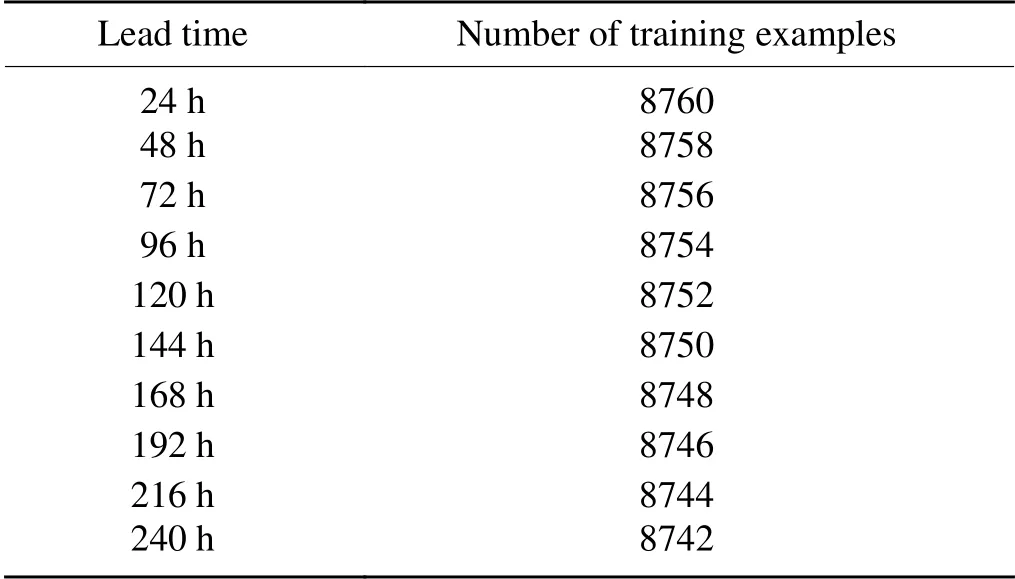

Table 1.Statistics of the training,validation,and testing datasets for 10 models.There are 730 validation and 730 testing examples for each lead time.

3.Methodology

We first explain how we transformed the forecast correction problem into an image-to-image translation problem in deep learning.It should be noted that all products used in this study are gridded data,which are similar to pixel-based images.The 2m-T correction problem is taken as an example in this section since the correction of other products essentially follows the same procedure.Given the 24 h forecast pof the 2m-T at the issue time t and the observation data yat t+24 h,we need to determine the mapping relationship f between pand y.Here,we use the deep learning method to obtain the solution of f.

Considering that the observation data of 2m-T yat the issue time t is closely related to y,it is also used as input to the deep learning network.The relationship between yand pand yis expressed as follows:

Figure 2

shows the flowchart of the deep learningbased bias correction method developed in this study.During the training period,historical 24-h ECWMF-IFS forecasts of the 2m-T and the observation data (ERA5) at the issue time t are fed into the deep network to train the CUnet model.The observation data (ERA5) at t+24 h is used as the ground truth during training.The trained CU-net is then used to correct new forecast data.

In the following sections,the basic concept of the CNN is briefly reviewed,and the construction of the CU-net model is detailed.In addition,the ANO method is briefly introduced as an existing traditional correction method,which is used for comparison.

3.1.Deep learning model

The basic structure of the CU-net model proposed in this study is similar to U-net,which is based on CNN.A standard CNN consists of convolution,pooling,fully connected,and activation layers (

Zeiler and Fergus,2014

).The convolution kernel of the convolution layer is similar to the filters used in image processing,such as the Sobel and Roberts filters,which have pre-determined weights known to be good for a certain operation (e.g.,smoothing or edge detection).However,the weights of the convolution kernel in the CNN are learned autonomously through network training.The output of a convolution layer is a feature map.Pooling is a downsampling operation,often inserted between two convolutional layers.Pooling layers allow shallow convolutional layers to learn fine-scale features and deeper convolutional layers to learn large-scale features.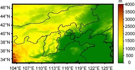

Fig.1.Study domain.The color bar stands for the terrain altitude.

Compared to traditional convolutional networks,U-net has a large number of feature channels in both downsampling and upsampling parts,resulting in a u-shaped network architecture as shown in

Fig.3

.The downsampling side is constructed by stacking downsampling convolutional modules (downconv) on the left side,and the upsampling side is constructed by stacking upsampling convolutional modules (upconv) on the right side.Different layers receive data with different spatial resolutions on two sides.The downconv modules accomplish the encoding process,which combines low-level features to obtain highlevel features.High-level features have a higher level of abstraction as they have passed through more convolutions and non-linear activations,but also a coarser spatial resolution due to the pooling operation.The downsampling and upsampling factors in this study are always 2 (i.e.,always either halve or double the spatial resolution).

The upconv modules perform the decoding process,which reconstructs the compressed information layer by layer and finally transforms it into predictions.The encoding and decoding processes are necessary because they turn the images into high-level features,which are better predictors than using raw pixel values,then they transform highlevel features into final predictions.The input (pand y)is fed directly to a standard convolutional layer (conv),which is the first convolutional layer on the encoding side.On the decoding side,the last convolutional layer is used to output the correction result.It should be noted that the data flow through CU-net from the top left (i.e.,first layer) to the bottom,then to the top right (i.e.,last layer).The other convolutional layers on the decoding side deal with intermediate representations.The benefit of having so many intermediate representations is that different convolutional layers can detect features at different spatial resolutions.

The green arrows in

Fig.3

represent skip connections,which mean that the features in the encoding process are reused in the decoding process through the concat layer.The purpose of skip connections is to enable U-net to preserve fine-scale information from shallower layers.Without skip connections,U-net would amount to simple downsampling followed by simple upsampling,leading to worse predictions,because upsampling can never recover all the fine-scale information lost during downsampling,which means that U-net would destroy a lot of fine-scale information.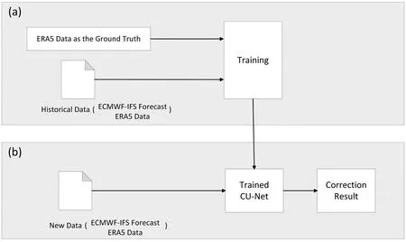

Fig.2.Flowchart of the deep learning correction method:(a) Model training,where historical 24 h ECWMF-IFS forecast and the observation data (ERA5) at time t-24 hours are fed into CU-net.The observation data (ERA5) at time t is used as the ground truth during training.(b) Model application.

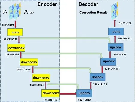
Fig.3.Architecture of the CU-net.The stacked downsampling convolutional modules (downconv) on the left side accomplish the encoding process,whereas the stacked upsampling convolutional modules (upconv) on the right side are responsible for the decoding process.The green arrows represent skip connections,which can preserve fine-scale information from shallower layers leading to better predictions.The data flow through the U-net from the top left to the bottom,then to the top right.

The detailed structures of downconv and upconv are shown in

Fig.4

,where downconv and upconv are mainly composed of convolution,pooling,and activation layers.The only change to U-net in this study is that “sub-pixel” is used to replace “interpolation” in the upconv module.

Shi et al.(2016)

has shown that “sub-pixel” is superior to “interpolation”,as the interpolation method only uses handcrafted filters for upsampling,whereas the sub-pixel layer is capable of learning a better and more complex mapping filter for upsampling.

In the upconv module,the sub-pixel layer is responsible for the upsampling operation,which increases the data resolution by r times (r is set to 2 in this study).Through a series of upconv modules,the network will finally yield 96×192 (lat×lon) images,which have the same size as the input (i.e.,the output grid has the same size as the input grid),which allows CU-net to make a prediction at every grid point.After data with a size of C × W × H pass through the sub-pixel layer,their size becomes (C × r × r) × W × H.Here,C represents the number of channels;W and H are the width and height of a feature map.Then the data are reshaped to C × (W × r) × (H × r),which leads to an increase in the data resolution by r times.The concat layer in the upconv module combines the features from the encoding process through a skip connection and the features from the decoding process through a sub-pixel operation.Assuming that the size of the feature map in the decoding process is C× W × H and the size of the feature map in the encoding process is C× W × H,the data size becomes (C+C) ×W × H after passing through the concat layer.The concat layer just appends the channels from the encoding process(skip connection) to the channels from the decoding process (sub-pixel operation).

As illustrated in

Fig.3

,the input of the network is the observation data of the 2-m temperature yand the 24 h forecast pof the 2m-T at the issue time t;the output is the corrected 24 h forecast pof the 2m-T.The observation data yat t+24 h is used as the ground truth during training.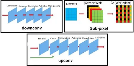

Fig.4.Illustration of the detailed structures of downconv,upconv,and sub-pixel.The concat layer appends the channels from the skip connection to channels produced by the sub-pixel operation.

Following the original U-net,the rectified linear unit(ReLU) is used as the activation function in CU-net (

Nair and Hinton,2010

).The ReLU function is defined as:f(x)=max(0,x).The convolution filter size is 3 × 3,which is commonly used.The Adam optimizer (

Kingma and Ba,2015

)and max pooling is used,and the pooling filter size is 2 × 2,which means that the pooling layer will always reduce the size of each feature map by a factor of 2.In this study,the number of epochs is set 50,which controls the number of complete passes through the training dataset.The learning rate is a hyper-parameter that controls how much to adjust the weights of the model with respect to the loss gradient.Typically,learning rates are set by the user,and it is often hard to get it right.Past experiences are often helpful to gain the intuition on what is the appropriate value.The learning rate is 0.001 in this study.Batch normalization is useful for training very deep neural networks,as it normalizes the inputs to a layer.Large neural networks trained on relatively small datasets tend to overfit to the training data,but the dropout technique can be used to mitigate this effect.As our model is not very large or deep,no batch normalization or dropout techniques are used.The number of CU-net parameters (i.e.,all the weights in the conv,upconv,and downconv layers) is 14,791,233.The loss function of the CUnet model is defined as mean squared error:

where y is the ground truth (i.e.,ERA5 data);y′ is the corrected forecast;and N is the number of grid points in one batch.To minimize the overhead and make maximum use of the GPU memory,the batch size,which indicates how many data samples are fed into the model for training at each time,is set to 32 in this study.Therefore,the size of N is 32×96×192.

In summary,CU-net has symmetric u-shaped network architecture.After the ECMWF-IFS forecast data are input to CU-net,its encoding process turns the images into highlevel features,which are better predictors than using lowlevel features or raw pixel values,then its decoding process transforms high-level features into final predictions.CU-net has many intermediate representations,whose benefit is that different convolutional layers can detect features at different spatial resolutions.It also uses skip connections to reuse the features from the encoding process in the decoding process to preserve fine-scale information from shallower layers.As the output grid has the same size as the input grid,CU-net is able to make a correction at every grid point.The above advantages are beneficial in correcting the forecast bias of numerical weather prediction models and make CUnet useful in this atmospheric application.

3.2.ANO method

As a traditional correction method,the ANO method is used for comparison with our CU-net technique in this study.The basic correction process of ANO is as follows.Given the coordinates (i,j) of a grid point,the model climate mean at (i,j) (i.e.,the average value of all pin n years) is given by:

The climate mean of observations is given by:

The corrected value is as follows:

where prepresents the corrected forecast value at (i,j);

p

represents the 24 h model forecast value at (i,j) in different years,

y

represents the observation data at (i,j) in different years,and n represents how many years of historical data are used.As the time window is 2005–16 in this study,n is equal to 12.For more details,please see

Peng et al.(2013)

.

4.Experiments and analyses

CU-net and ANO were used to correct the forecast of four weather variables from ECMWF-IFS:2m-T,2m-RH,10m-WS,and 10m-WD.For each weather variable,the corresponding correction performance is discussed according to different seasons.In this study,spring includes March,April,and May;summer corresponds to June,July,and August;autumn consists of September,October,and November;and winter includes December,January,and February.

We use the root mean square error (RMSE) to evaluate the correction performance,which is defined as:

where T represents the number of samples in the testing dataset;M represents the length of the study domain on the xaxis;and N represents the width of the study domain on the y-axis.

p

represents the forecast value or corrected value at (i,j) at the forecast issue time t,and

y

represents the observation value of (i,j) at t.T is 730,M is 192,and N is 96 in this study.

According to the China Meteorological Administration’s standard “QXT 229–2014 Verification Method for Wind Forecast,” the RMSE (in degrees) of wind direction is defined as follows:

The bootstrap method for significance test was used in this study.The null hypothesis is that the correction method provides no improvement over ECMWF-IFS.First,setting R as the number of bootstrap replicates (1000 in our case)and N as the number of examples in testing data,R bootstrap replicates of the testing data were created.Then,for each bootstrap replicate,the difference between the models in the score of interest (e.g.,RMSE for CU-Net minus RMSE for ECMWF) was calculated.Finally,these R values of the difference in the score of interest were used to perform significance testing at the 95% level.In this study,all the confidence intervals at the 95% level were also created with bootstrapping.

4.1.Correction results for 2m-T

Figure 5

shows the RMSE spatial distribution of the corrected 24 h forecast for 2m-T in all seasons in 2018.Significance tests were conducted on the data for the whole year,and significant grid points (at the 95% confidence level) are represented in

Fig.5

with stippling.The forecast RMSE of ECMWF-IFS (as shown in the left column of

Fig.5

) is relatively large in spring and winter,and smaller in summer and autumn;the error over the ocean is very small,whereas the error over complex terrain is relatively large.Both ANO (middle column of

Fig.5

) and CU-net (right column of

Fig.5

) had smaller RMSE than raw IFS output;however,CU-net outperformed ANO in every season,as well as for the whole year.Over areas with complex terrain,the RMSE of the ANO method exceeded 2.0°C,whereas CU-net reduced this to about 1.5°C.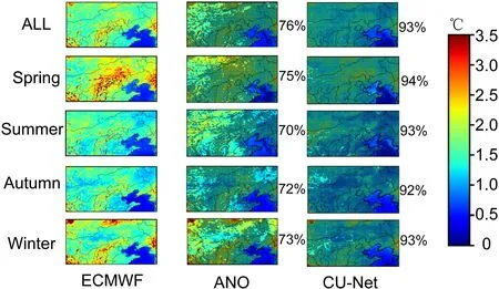

Fig.5.Root mean square error (RMSE) distributions of the corrected 24 h forecast of 2m-T in different seasons in 2018.The left column represents the forecast errors of ECMWF,whereas the middle and right columns are for corrected product based on ANO and CU-net,respectively.In each panel,points with stippling denote places where differences with respect to ECMWF-IFS are statistically significant at the 95% level.The number on the right represents the percentage of stippled points in all points,which means the correction methods provide improvement over ECMWF-IFS on these grid points.

Figure 6 a

shows the RMSE values for temperature for each model in different seasons.CU-net had smaller RMSEs than ANO,which also outperforms ECMWF-IFS.In all seasons,CU-net outperforms ANO and ECMWF-IFS.

Table 2

shows the bias,mean absolute error (MAE),correlation coefficient,and RMSE values of the corrected 24 h forecast for 2m-T in 2018 using ECMWF,ANO,and CU-net.The confidence intervals are at the 95% confidence level.ANO achieves better performance than ECMWF-IFS,but CU-net has the best performance in terms of all evaluation metrics.

Figure 7

shows an example 24 h forecast case at 1200 UTC on 11 January 2018.It is obvious that the corrected result using CU-net is more consistent with the observation(ERA5).It should be noted that ERA5 is reanalysis data,which is smoother than ECMWF and ANO.As CU-net uses ERA5 as the ground truth to perform correction,its result also seems smooth.For longer-term forecasts of 2m-T,

Fig.8

shows the change in the RMSE of CU-net and ANO according to different forecast lead times (24–240 h).CU-net achieved the smallest RMSE for all forecast lead times.Even for the 240 h forecast,CU-net had a percentage decrease of 10.75%,compared to almost 0% for ANO.

4.2.Correction results for 2m-RH

Figure 9

shows the RMSE spatial distribution of the corrected 24 h forecast for 2m-RH.The same significance tests as in

Fig.5

were conducted for the data from different seasons.Compared to the ECMWF results in the left column of

Fig.10

,both ANO and CU-net exhibited improved forecast accuracy;however,CU-net was superior to ANO for every season,as well as for the entire year.In

Fig.9

,the area marked in red represents a large RMSE of about 0.14.For the winter season,over the red areas,we can see that ANO and CU-net reduced the RMSE to 0.12 and <0.1,respectively.

Figure 6b

shows the RMSE values for each model in different seasons for 2m-RH.The confidence intervals are at the 95% confidence level.ANO achieved positive correction performance in spring,autumn,and winter,but had negative performance during the summer.By contrast,CU-net achieved better performance in all seasons than ANO and ECMWF-IFS.

Table 3

shows the bias,MAE,correlation coefficient,and RMSE values of the corrected 24 h forecast for 2m-RH.CU-net achieved the best performance for all four evaluation metrics.

Table 2.Bias,MAE,correlation coefficient (CC),and RMSE of the corrected 24 h forecast for 2m-T.The confidence intervals are at the 95% confidence level.

Figure 10

shows an example 24 h forecast case at 1200 UTC on 19 October 2018,to illustrate that the corrected result using U-net is more consistent with the observation(ERA5).For longer-term forecasts of 2m-RH,

Fig.11

shows the change in the RMSE of CU-net and ANO,according to different forecast lead times (24–240 h).Similar to the results of the 2m-T correction discussed above,CU-net achieved the smallest RMSE for all forecast lead times.For the 240 h forecast correction,ANO showed a percentage decrease of–2.26% compared to 20.14% for CU-net.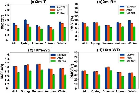

Fig.6.RMSE of the corrected 24 h forecast in all seasons in 2018 for 2m-T (a),2m-RH (b),10m-WS (c),and 10m-WD (d).The confidence intervals at the 95% confidence level are shown with black error bars.

4.3.Correction results for 10m-WS

Figure 12

shows the RMSE spatial distribution of the corrected 24 h forecast for 10m-WS.Significance tests were also conducted in the same way as in

Fig.5

.Compared to the results of ECMWF in the left column of

Fig.12

,ANO showed no improvement,whereas CU-net showed obvious improvements in all seasons.

Figure 6c

shows the RMSE values for each model in different seasons for 10m-WS.ANO improved over the ECMWF only in autumn and had negative performance for all other seasons,whereas CU-net achieved improvement in all seasons.

Table 4

shows the bias,MAE,correlation coefficient,and RMSE values of the corrected 24 h forecasts for 10m-WS using ECMWF,ANO,and CU-net.The confidence intervals are at the 95% confidence level.Again,CUnet has the best correction performance in terms of all evaluation metrics.

Table 3.Same as Table 2 but for 2m-RH.

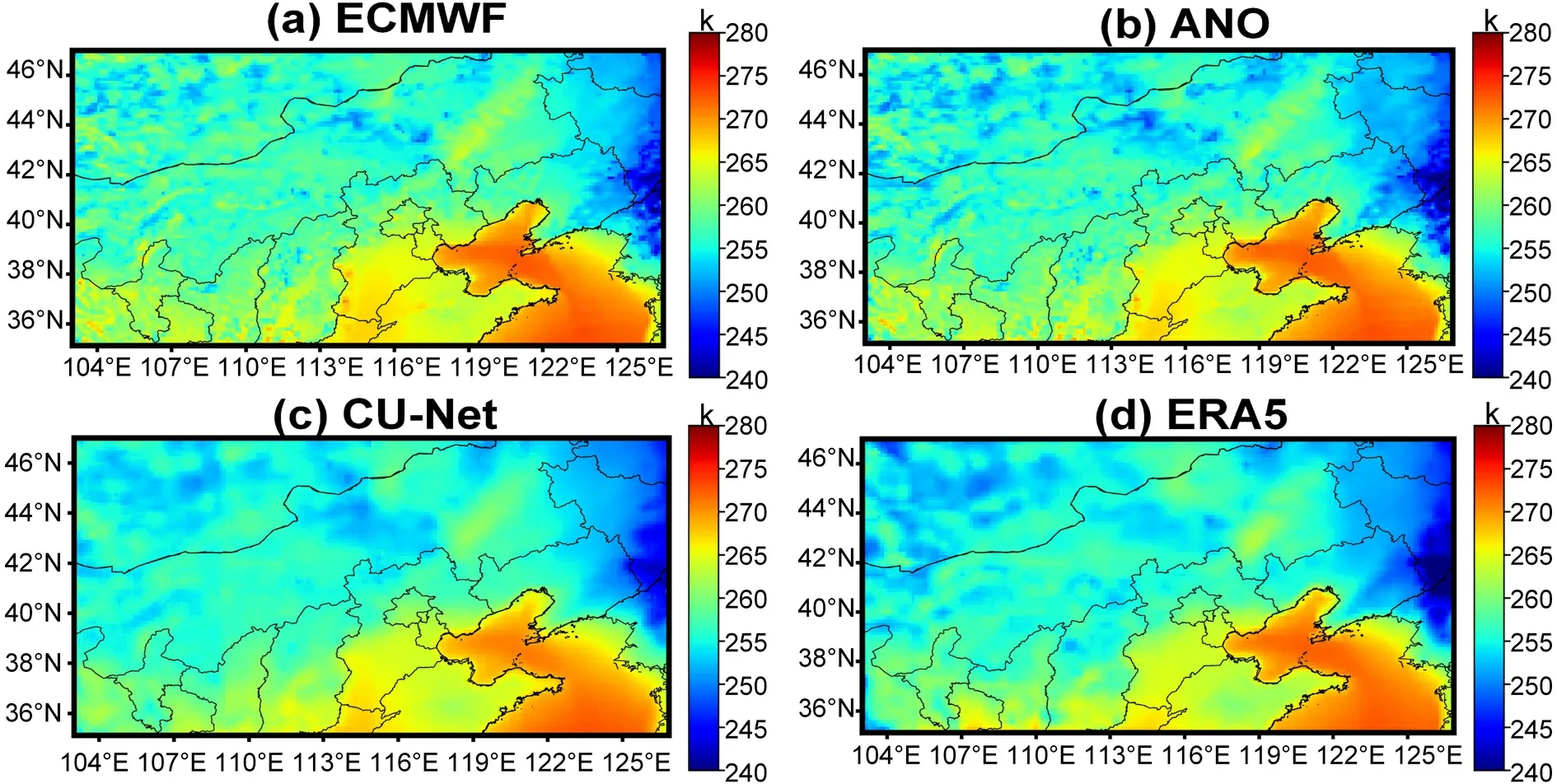
Fig.7.Illustration of 24 h 2m-T forecast at 1200 UTC on 11 January 2018:(a) ECMWF;(b) corrected forecast using ANO;(c) corrected forecast using CU-net;(d) ERA5.

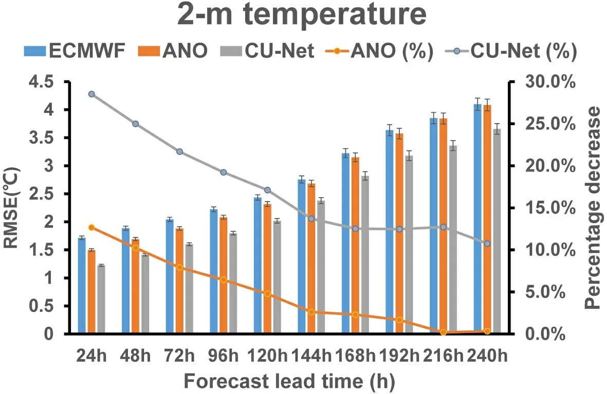
Fig.8.Change in the RMSE of the corrected 24 h forecast for 2m-T with respect to different forecast lead times.The evaluation was performed on the testing data (2018).The confidence intervals at the 95% confidence level are shown with black error bars.

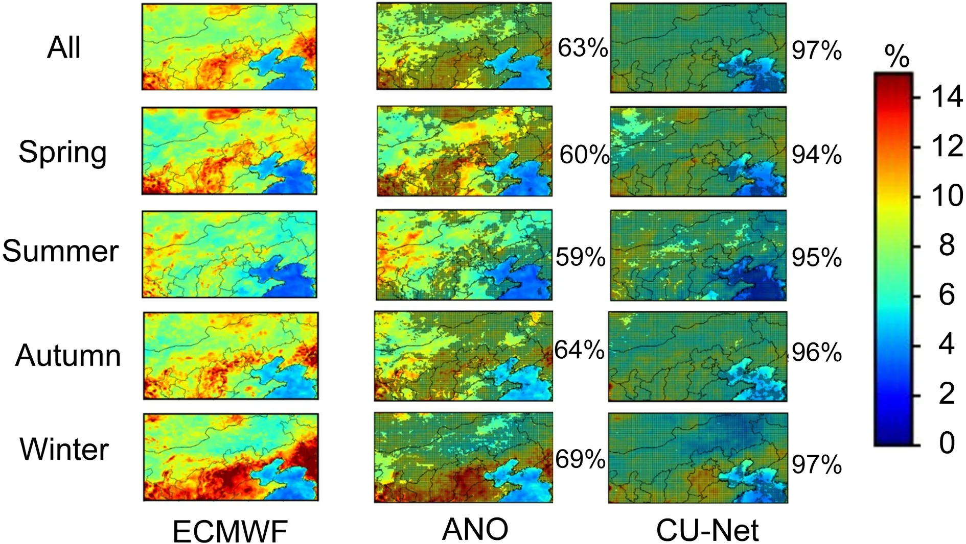
Fig.9.Same as Fig.5,but for 2m-RH.

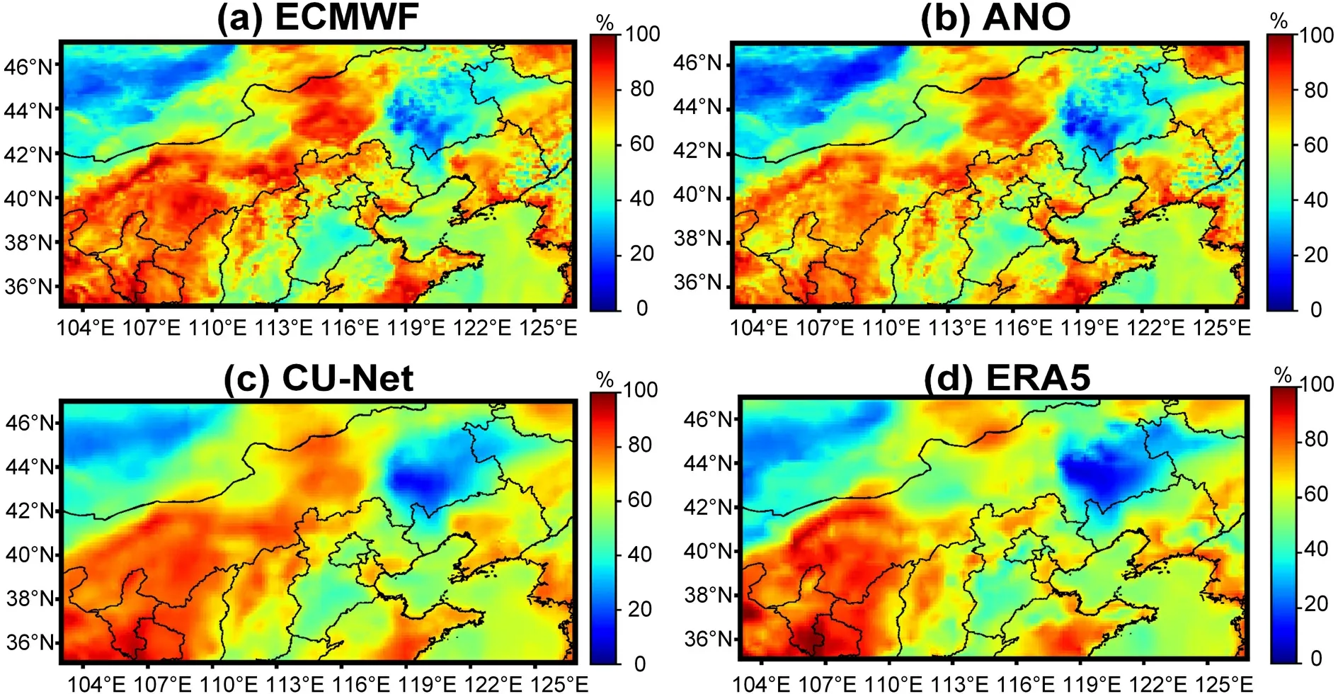
Fig.10.Illustration of 24 h 2m-RH forecast at 1200 UTC on 19 October 2018:(a) ECMWF;(b) corrected forecast using ANO;(c) corrected forecast using CU-net;(d) ERA5.

Figure 13

shows the 24 h forecast on 15 March 2018,and therein the red ellipse indicates that ECMWF and ANO have obvious error while CU-net’s correction is more consistent with the observations.For longer-term forecasts of 10m-WS,

Fig.14

shows the change in the RMSEs of CU-net and ANO,according to the forecast lead time.Similar to the results of 2m-T and 2m-RH correction,CU-net achieved the smallest RMSE for all forecast lead times.In general,ANO did not perform well for 10m-WS forecast correction.For all different forecast lead times,ANO did not have a positive correction effect.CU-net continued to provide positive results as theforecast lead time approached 240 h.

4.4.Correction results for 10m-WD

Figure 15

shows the RMSE spatial distribution of the corrected 24 h forecast for 10m-WD.Significance tests were also conducted in the same way as in

Fig.5

.Similar to the results for 10m-WS correction,ANO showed no improvement and in some cases showed worse results.CU-net showed improvements in all seasons.Notably,the correction of wind direction has been a challenging issue,as described in previous studies (

Bao et al.,2010

).

Figure 6d

shows the RMSE values for each model in different seasons for 10m-WD.ANO did not show a positive performance in any season.By contrast,CU-net achieved a positive performance in all seasons.

Table 5

shows the bias,MAE,correlation coefficient,and RMSE values of the corrected 24 h forecast for 10m-WD.The confidence intervals are at the 95% confidence level.

Figure 16

shows the forecast results on 18 April 2018.Similar to previous experiments,CUnet’s correction is more consistent with the observation although it has a smoothing effect.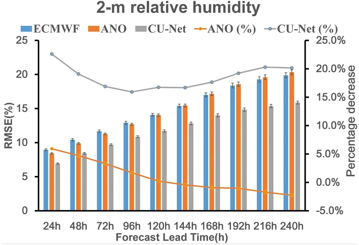

Fig.11.Same as Fig.8,but for 2m-RH.

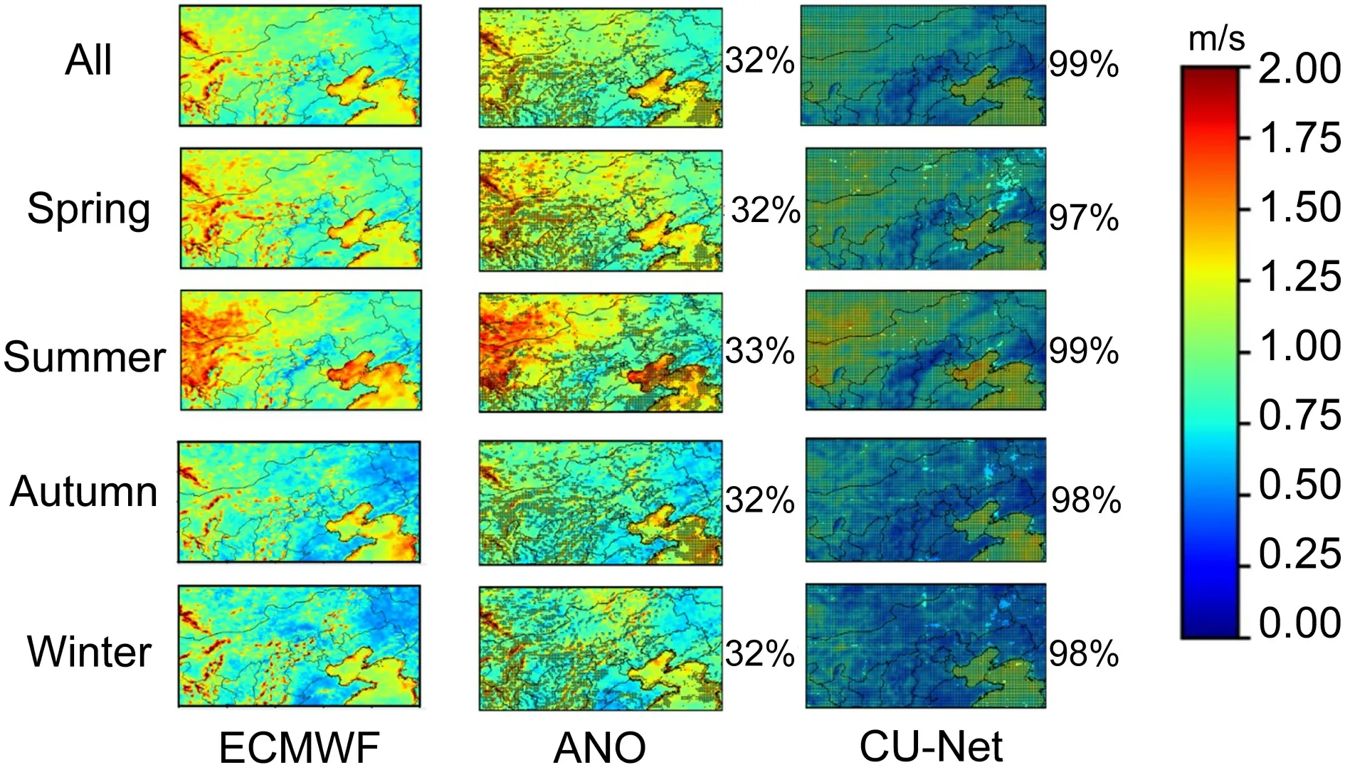
Fig.12.Same as Fig.5,but for 10m-WS.

Table 4.Same as Table 2 but for 10m-WS.

For longer-term forecasts of 10m-WD,

Fig.17

shows the change in the RMSE of CU-net and ANO according to different forecast lead times.Again,CU-net achieved the smallest RMSE for all forecast lead times.Similar to the 10m-WS correction,ANO did not perform well for the 10m-WD forecast correction and did not have a positive correction effect for any lead time.Although CU-net continued to provide positive results as the forecast lead time increased,its performance continued to degrade from 18.57% (24 h) to 3.7% (240 h).

4.5.Using reliability curves for conditional forecast verification

In order to identify if CU-net has conditional bias,we use reliability curves to further evaluate its performance for each forecast value.The 24 h forecast results are used for analysis.As shown in

Fig.18

,the reliability curve has forecast values on the x-axis and mean observation on the y-axis.The black line is the perfect-reliability line (x=y) which represents the observation ERA5 (correct answers).

Figures 18a

and

b

show that for 2m-T and 2m-RH,CUnet performs better than other methods.For 10m-WS,as shown in

Fig.18c

,CU-net achieves overall good performance,though there are slight underestimations whenever it predicts >～6.5 m s.For 10m-WD,

Fig.18d

shows that CUnet obviously fits better with the diagonal line than other models.Besides,all panels show that each model has conditional bias,while CU-net has smallest bias.

4.6.Correction results after incorporating terrain information

This section describes an additional experiment that was conducted to test whether including terrain information in the proposed CU-net model could offer further improvements in the correction (

Steinacker et al.,2006

).The terrain data Q (a grid of orographic height),along with pand y,were input into the CU-net model,as shown in

Fig.3

;the new model with terrain data is referred to as TCU-net.The experimental results of the 24 h forecast correction are shown in

Table 6

.The confidence intervals are at the 95%confidence level.It can be seen that TCU-net improved the performance,as all four weather variables showed smaller RMSEs after including the terrain information.

Table 5.Same as Table 2 but for 10m-WD.

Table 6.RMSE of the corrected 24 h forecast in 2018 for four weather variables using ECMWF,CU-net,and TCU-net.The confidence intervals are at the 95% confidence level.

4.7.Discussion

Some studies have shown that the ANO method has more stringent requirements on the length of the time period of the data (

Chang et al.,2015

).In this study,we used 14 years of data.Using longer-term data may help improve the correction performance of ANO.It also should be mentioned that,for the ANO method,each grid point remained independent during the correction process.However,weather phenomena are continuous not only in time but also in space (i.e.,each grid point is impacted by its neighboring grid points).Hence,it is necessary to take these spatial impacts into account,which happens to be the strength of CNN since it inherently learns the spatial information through the convolution operations.In general,the above factors explain the limited performance of ANO compared to CU-net.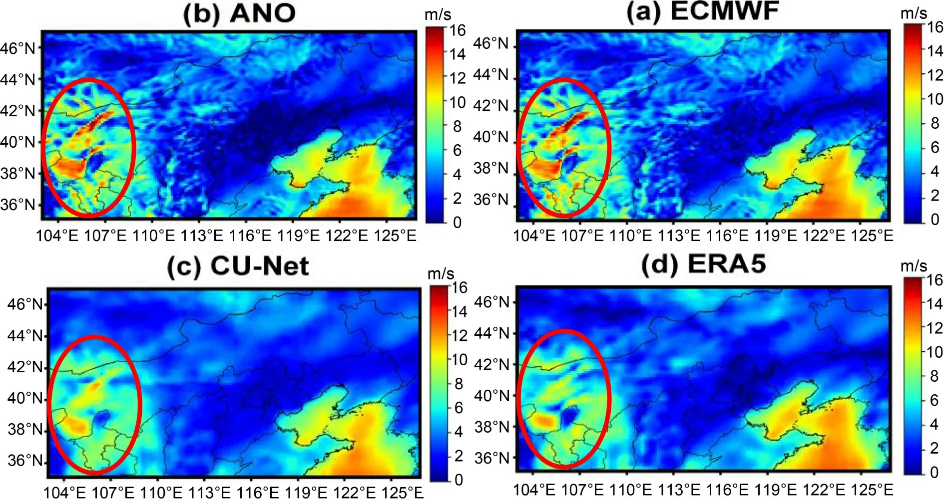

Fig.13.Illustration of 24 h 10m-WS forecast at 1200 UTC on 15 March 2018:(a) ECMWF;(b) corrected forecast using ANO;(c) corrected forecast using CU-net;(d) ERA5.The red ellipse indicates that ECMWF and ANO have obvious error while CU-net’s correction is more consistent with the observations.

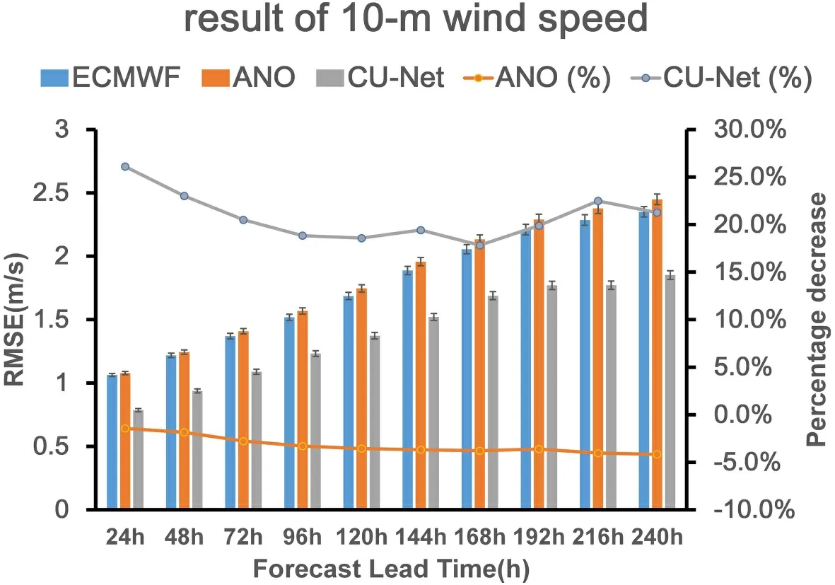
Fig.14.Same as Fig.8,but for 10m-WS.

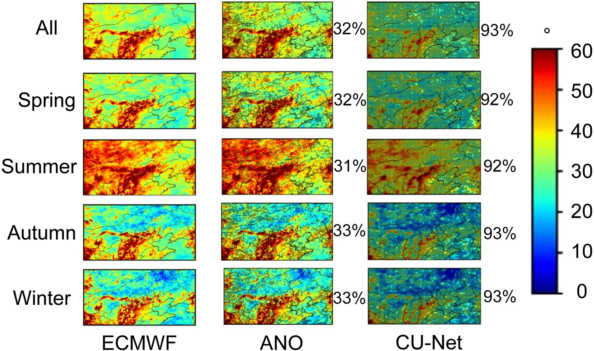
Fig.15.Same as Fig.5,but for 10m-WD.

5.Summary

This study first transformed the forecast correction problem into an image-to-image translation problem and then proposed a CU-net model based on CNNs.Fourteen years of ECMWF-IFS forecast data and ERA5 data (2005–2018)were used for training,validation,and testing;specifically,the 2005–2016 data were used as the training dataset,the 2017 data as the validation dataset,and the 2018 data as the testing dataset.We used the proposed CU-net as well as a traditional correction method (i.e.,ANO) to correct the forecast of four weather variables from ECMWF-IFS:2m-T,2m-RH,10m-WS,and 10m-WD,and compared their performance.The experimental results showed that CU-net had a smaller RMSE than ANO for all variables and for all forecast lead times from 24 h to 240 h.CU-net improved uponthe ECMWF-IFS forecast for all four weather variables,whereas ANO improved upon ECMWF-IFS performance for only 2m-T and 2m-RH.For the difficult problem of 10m-WD forecast correction,although it is worse than 2m-T,2m-RH,and 10m-WS,CU-net still achieved a percentage decrease of 18.57% for 24 h correction and 3.7% for 240 h correction.In comparison,ANO gave negative correction results for the 10m-WD forecast.Considering the impact of terrain on weather forecasting,we added an additional experiment to test whether including terrain information in CU-net would improve the correction.The results of the 24 h forecast correction showed that all four weather variables had a smaller RMSE after incorporating the terrain information.

The impact of time dimension was not considered in this study.Incorporating a time component into the model(e.g.,by using LSTM) may further improve the model’s performance.It may be a potential direction for future study.Using more fields as predictors in the model is another worthy idea to try for future study.

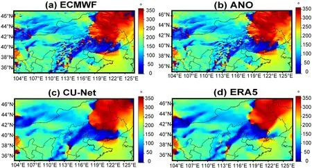
Fig.16.Illustration of 24 h 10m-WD forecast at 1200 UTC on 18 April 2018:(a) ECMWF;(b) corrected forecast using ANO;(c) corrected forecast using CU-net;(d) ERA5.

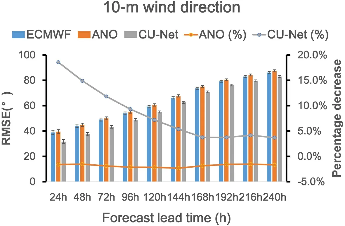
Fig.17.Same as Fig.8,but for 10m-WD.

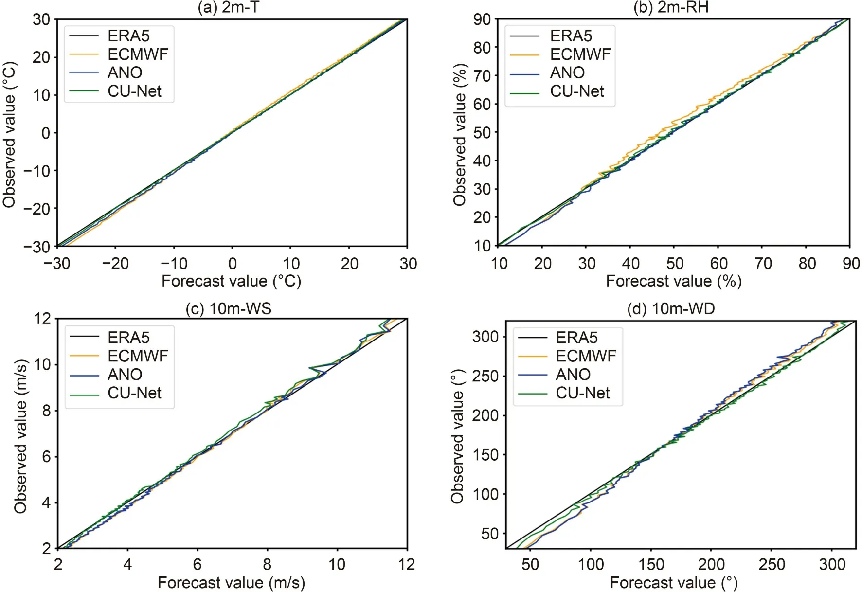
Fig.18.Reliability curves of the corrected 24 h forecast in 2018 for 2m-T (a),2m-RH (b),10m-WS (c),and 10m-WD (d).

.This work was supported in part by the National Key R&D Program of China (Grant No.2018YFF0300102),the National Natural Science Foundation of China (Grant Nos.41875049 and 41575050),and the Beijing Natural Science Foundation (Grant No.8212025).We gratefully acknowledge the support of NVIDIA Corporation for the donation of the GPU used for this research.This article is distributed under the terms of the Creative Commons Attribution License which permits any use,distribution,and reproduction in any medium,provided the original author(s) and the source are credited.This article is distributed under the terms of the Creative Commons Attribution 4.0 International License (

http://creativecommons.org/licenses/by/4.0/

),which permits unrestricted use,distribution,and reproduction in any medium,provided you give appropriate credit to the original author(s) and the source,provide a link to the Creative Commons license,and indicate if changes were made.