Spatial prediction and modeling of soil salinity using simple cokriging,artif icial neural networks,and support vector machines in El Outaya plain,Biskra,southeastern Algeria
Samir Boudibi·Bachir Sakaa·Zineeddine Benguega·Haroun Fadlaoui·Tarek Othman·Narimen Bouzidi
Abstract Soil salinization is one of the most predominant environmental hazards responsible for agricultural land degradation,especially in the arid and semi-arid regions.An accurate spatial prediction and modeling of soil salinity in agricultural land are so important for farmers and decision-makers to develop the appropriate mechanisms to prevent the loss of fertile soil and increase crop production.El Outaya plain is marked by soil salinity increases due to the excessive use of poor groundwater quality for irrigation.This study aims to compare the performance of simple kriging,cokriging(SCOK),multilayer perceptron neural networks(MLP-NN),and support vector machines(SVM)in the prediction of topsoil and subsoil salinity.The f ield covariates including geochemical properties of irrigation groundwater and physical properties of soil and environmental covariates including digital elevation model and remote sensing derivatives were used as input candidates to SCOK,MLP-NN,and SVM.The optimal input combination was determined using multiple linear stepwise regression(MLSR).The results revealed that the SCOK using f ield covariates including water electrical conductivity(ECw)and sand percentage(sand%),and environmental covariates including land surface temperature(LST),topographic wetness index(TWI),and elevation could signif icantly increase the accuracy of soil salinity spatial prediction.The comparison of the prediction accuracy of the different modeling techniques using the Taylor diagram indicated that MLP-NN using LST,TWI,and elevation as inputs were more accurate in predicting the topsoil salinity[ECs(TS)]with a mean absolute error(MAE)of 0.43,root mean square error(RMSE)of 0.6 and correlation coeff icient of 0.946.MLP-NN using ECw and sand%as inputs were more accurate in predicting the subsoil salinity[ECs(SS)]with MAE of 0.38,RMSE of 0.6,and R of 0.968.
Keywords Soil salinity·Cokriging·Multilayer perceptron·Machine learning·El-Outaya plain
1 Introduction
Soil salinization is def ined as the process of salt enrichment in the soil,which can be caused by two different factors as natural(primary salinization)salty groundwater table near the soil surface(upwelling)and/or human-induced(secondary salinization)irrigation with saline water that leads to the increase of salts’accumulation in the irrigated lands(Pouladi et al.2019;Koulla et al.2019).Soil salinity is one of the major environmental hazards that cause land degradation and affects agricultural productivity and the sustainability of land resources all over the world.The secondary salinization affects almost 45 million ha(20%)of the total cultivated and 74 million ha(33%)of irrigated agricultural areas in the world(Shrivastava and Kumar 2015).Furthermore,the salinized areas are still increasing at a rate of 10%each year due to different problems including high surface evaporation,low precipitation,chemical or physical weathering of native rocks,irrigation with high saline water,and poor cultural practices(traditional irrigation techniques practiced with irrelevant drainage systems)(Gorji et al.2020).Some researchers estimated that 50%of the world’s arable land will be affected by salinity(Machado and Serralheiro 2017).
In the Mediterranean region,the salt-affected soil is estimated at 1 million ha and it is the main cause of desertif ication(Machado and Serralheiro 2017).Algeria is one of the Mediterranean countries,where agricultural land is largely affected by this phenomenon,especially in the southeastern part of the country such as Biskra province,which is characterized by an arid climate and groundwater is the main source of irrigation.The farmers of this region are using poor quality groundwater,usually unsuitable for irrigation,and characterized by high salinity(Boudibi et al.2019,Abdennour et al.2020).Such practice has enhanced the development of the agricultural sector,but it is also a principal factor of soil salinization.It is urgent and necessary to ascertain the best modeling technique to improve the soil salinity prediction by using auxiliary variables,which can enhance the ability of decision-makers and landuse planners to assess accurately the soil salinity and to reduce the cost and time-consuming sampling campaigns.
Many tools,modeling techniques,and spatial interpolation methods have been developed and applied by researchers for the spatiotemporal monitoring and assessment of soil properties,especially soil salinity in terms of soil electrical conductivity(ECs).Numerous geostatistical techniques have been applied for the spatiotemporal predictions of soil salinity and soil properties,including ordinary Kriging(Dai et al.2014;Shahabi et al.2016;Koulla et al.2019),indicator kriging(Bradaı¨et al.2016),and cokriging (Shen et al.2019).Recently,many researchers also applied new machine learning methods to predict soil characteristics.Were et al.(2015)used artif icial neural networks(ANN),support vector machine(SVM),and random forest(RF)for predicting and mapping soil organic carbon stocks in Kenya.Achieng(2019)applied an artif icial and deep neural network for modeling soil moisture and Pouladi et al.(2019)used multilayer perceptron neural network(MLP-NN)for predicting soil salinity in Iran.All the mentioned studies have shown the high accuracy of machine learning techniques in modeling soil properties.
The main purpose of this paper is to improve the prediction of soil salinity by the integration of new f ield and environmental covariates and explore the most suitable auxiliary variables for soil salinity prediction using multiple linear stepwise regression(MLSR).Finally,the evaluation and comparison of various model performance are presented including simple kriging(SK),simple cokriging(SCOK),multilayer perceptron neural network(MLP-NN),and support vector machine(SVM)modeling techniques in predicting the variability of ECs in El Outaya plain,southeastern Algeria using mean absolute error(MAE),root mean square error(RMSE),correlation coeff icient(R),determination coeff icient(R)and Taylor diagram.
2 Materials and methods
2.1 Study area
The current study was performed in El Outaya plain in Biskra province,southeastern Algeria(Fig.1).The study zone is located between 34°48-35°03N latitude and 5°09-5°45E longitude and covers an area of 40500 ha.From the morphological and bioclimatic points of view,the Biskra region can be considered a transition zone between the northern and southern parts of Algeria(Abdennour et al.2020).The study area lies in an arid climate with average annual precipitation,which seldomly exceeds 150 mm,average annual evaporation often is in excess of 2500 mm and a mean temperature ranges from 11°C in the coldest month(January)to 35°C in the hottest month(July).

Fig.1 Location of the study area and soil samples
El Outaya plain is characterized by an irrigated agriculture and the groundwater is the main source of irrigation despite the existence of Gazelles’Fountain dam,which is used only for the irrigation of El Hzima perimeter that is located near to Djebel Boughezal in the southern part of the study area.The crop patterns vary considerably in the study area due to the small size of farms,where cereals,alfalfa and olive cultures are the dominant production systems,because of their tolerance to high levels of water and soil salinity.
The main hydrogeological units in El Outaya plain are the Lower Eocene,the Mio-Pliocene,and the quaternary(Boudjema 2015).The Mio-Pliocene is the main exploited aquifer in El Outaya plain.The water quality of this aquifer is good to permissible for irrigation in the east and the west of the study area,while it is poor and unsuitable for irrigation in the middle(Boudibi et al.2019).The irrigation with the saline groundwater of this aquifer is associated with high evaporation enhancing the secondary soil salinization and the accumulation of soluble salts into the soil surface.
According to the soil map of Algeria,Biskra,produced by Durand and Barbut(1938)and explained by Benchetrit(1956),El Outaya plain is characterized by basic alluvium surrounded by wind ablation soils.Saline soils(Slontchak type)are present in the synclinal depression of Selga Saadoun.The western part of the plain is characterized by wind accumulation soils(dunes)due to wind erosion.
2.2 Soil sampling and ECs analysis
A total of 136 soil samples are collected from 68 irrigated farms in El Outaya plain from 20 May to 20 June 2018.At each irrigation farm,two soil depths(topsoil at 0–20 cm and subsoil of 40–60 cm)are sampled using a hand auger and placed into polyethylene bags.In the laboratory,the samples are air-dried,crushed,and sieved through a 2 mm sieve.The soil particle fractions(clay,sand,and silt)is determined using the pipette method.The soil electrical conductivity(ECs)is measured in a 1:5 soil water diluted extract method using the multi-parameter(WTW multi 3430).The measured ECs are used to express the soil salinity.
2.3 Covariates collection
The covariates used for prediction and soil salinity modeling are continuous variables and they are regrouped into two categories,namely,the f ield measurement and the environmental covariates.The f ield measurements covariates include irrigation water and soil properties,and the environmental covariates includes DEM derivatives and remote sensing derivatives are used for modeling soil salinity in El Outaya plain.Therefore,80%of the samples,distributed throughout 54 sampling locations,are used for training and 20%,distributed over 14 sampling locations are used for testing the different modeling techniques.The used methodologies are summarized in Fig.2.
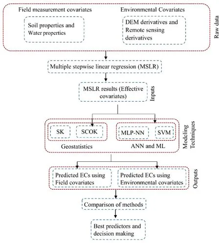
Fig.2 Flowchart of the used methodology
2.3.1 Field measurement covariates
The irrigation water properties are obtained from 68 groundwater samples(the same distribution of the soil samples).The used water properties are the electrical conductivity of groundwater(ECw),the potential Hydrogen(pH),cations plus anions of groundwater,the sodium percentage(Na%),the sodium adsorption ratio(SAR).The soil properties covariates are the soil particle fractions(clay%,sand%and silt%)of the topsoil and subsoil.
2.3.2 Environmental covariates
The digital elevation model(DEM)derivatives are used for modeling soil salinity including elevation,aspect,curvature,slope and topographic wetness index(TWI)(Fig.3).These DEM derivatives are calculated using ArcGis 10.2.The 30 m resolution Shuttle Radar Topography Mission(SRTM)DEM data covers the entire study area,and they are obtained from the United States Geological Survey(USGS)website.

Fig.3 The raw covariates derived from DEM:a elevation b slope c TWI d aspect e curvature
The remote sensing derivatives are generated using Landsat-8 OLI satellite images.A Landsat-8 satellite image with 30 m of resolution dated on the same period of soil and groundwater sampling(12 June 2018)is obtained by downloading from the USGS website.The Landsat-8 OLI image is atmospherically corrected and radiometrically calibrated using ENVI 5.3 software through the FLAASH atmospheric model.After mosaicking and clipping the satellite image,three derivatives are calculated including the Land Surface Temperature(LST),the Normalized Difference Vegetation Index(NDVI)and Soil Adjusted Vegetation Index(SAVI)by using map algebra tool of ArcGis software(Fig.4).

Fig.4 The raw covariates derived from satellite images:a NDVI,b SAVI,c LST
The NDVI is a standardized index that allows the relative biomass map generation.The default equation of NDVI is as follows(Shen et al.2019):

where NIR and R are the near-infrared and Red bands of the Landsat-8 image,respectively.
The SAVI is a vegetation index used in regions with low vegetative cover(arid regions),where it attempts to minimize the inf luence of soil brightness(ESRI 2020).It is calculated as follows(Huete 1988):

where L is the soil brightness correction factor,which depends on the amount of green vegetation cover(0.5 in this study).
The LST is one of the most important aspects of the land surface calculated from remote sensing.It is def ined as the skin temperature of the ground(Avdan and Jovanovska 2016).The LST is computed as follows(Avdan and Jovanovska 2016;Yin et al.2020):

where BT is at sensor brightness temperature from Eq.4(°C),λis the wavelength of emitted radiance(λ(band 10)=10.8μm),εis the emissivity calculated using Eq.(5)andρ=h*c/δ=1.4388*10m k;h is the Plank’s constant(h=6.626*10),c is the velocity of light(c=2.998*10m/s)andδis the Boltzmann’s constant(δ=1.38*10).

where Lrepresents the top of atmosphere spectral radiance(Eq.6),Kand Kare the band specif ic thermal conversion constants from the metadata f ile,respectively.

where Mis the band-specif ic multiplicative rescaling factor,Qthat represents the band 10 of the satellite image and Ais the band-specif ic additive rescaling factor.
2.4 Covariates preprocessing
Regression techniques,such as multiple linear stepwise regression(MLSR),are often used to predict a dependent variable(response)by using one or more independent variables(predictors).In the case of a high number of covariates,it is essential to select the most important covariates for modeling(Zounemat-kermani and Scholz 2014).MLSR is a combination of forwarding selection and
backward elimination of input variables to generate the best combinations to the model(Zounemat-Kermani et al.2020).The probability of F statistic(pF)for inclusion is set at 0.05(if pF is less than 0.05,the auxiliary variable will be included in the linear equation)and the pF statistic for exclusion is set at 0.1(if pF is greater than 0.1,the auxiliary variable will be excluded)(Gu et al.2017).Some covariates are found correlated between themselves,which are referred to as multicollinearity and the covariates should be independent variables(Jalal et al.2020).MLSR is an available method for eliminating multicollinearity problem between the covariates(Shen et al.2019).In this study,MLSR is used for determining the optimal input combinations for SCOK,MLP-NN and SVM modeling techniques.
2.5 Modeling techniques
2.5.1 Simple kriging(SK)
Simple Kriging (SK)estimator is considered as the weighted linear combination in which,the areal mean of the regionalized variables is known and must be secondorder stationary(mean and variance constancy)(Maroufpoor et al.2017;S¸en 2016).Simple Kriging equation can be written as,

x
)is the linear regression estimator,Z
(x
)is the regionalized variable at the locationx
,μis the locationdependent expected value ofZ
(x
),w
are the weights andμ is the mean of the SK process.2.5.2 Simple cokriging(SCOK)
Cokriging(COK)estimator is a developed multivariate extension of Kriging,where the aim is to predict one target variable using additional information of one or more axillary variables,which are correlated with the primary variable(Webster and Oliver 2007).Simple cokriging(SCOK)is a multivariate extension of simple Kriging.The SCOK estimator is made up of the target variable mean of interest plus a linear combination of weightsλwith the residuals of the auxiliary variables(Wackernagel 2003).SCOK is expressed as,


2.5.3 Multilayer perceptron neural network(MLP-NN)
The multilayer perceptron neural network(MLP-NN)is one type of Artif icial Neural Networks(ANNs)called a feed-forward neural network,which is the most commonly applied ANNs to solve environmental problems(Pouladi et al.2019;Sakaa et al.2020).In this study,MLP-NN is used for the prediction of soil salinity(ECs).The MLP-NN is structured with one input layer,one or more hidden layers(one layer in this study),and an output layer(Fig.5).The neurons of each layer are connected to the neurons of the subsequent layer through synaptic weights,but not in the same layer(Erdik et al.2009).The number of neurons in the hidden layer is determined after training and testing of a series of networks having from 1 to 20 neurons in order to obtain the best structure with minimum error(e.g.square of errors,SOS) and maximum correlation coeff icient.

Fig.5 Schematic representation of three-layered feed-forward MLP-NN
In MLP-NN,the input variables(x)are fed into the input layer neurons(x)which send them to the hidden layer(y).The neurons of the hidden layer sum up the received value of the input layer after the multiplication of each input value by its weight(w)and adding a bias(b).The weighted sum(S)becomes the input to activation function in the hidden layer,the latter generates the output of each neuron in the hidden layer,which in turn,becomes the input of activation function in the output layer,where the output variable(Z)is generated(Erdik et al.2009;Kisi et al.2017;Sakaa et al.2020).

S
is the weighted sum,b
is the bias,xstands for the input standardized value,n is the number of input variables in the input vector and wis the synaptic weights.The overall equation that describes the input/output relationship of three-layered MLP-NN is as follows(Bishop 1995):

Z
is one of the output variables,band bj are the bias(they can be absorbed into the weights),w
andw
denote successively the weights between the input layer and the output layer neurons and between the hidden layer and the output layer neurons,p
is the number of neurons in a hidden layer,n
is the number of neurons in the input layer,f
andf
are the activation functions of the neurons of the hidden layer and the neurons of the output layer,successively.In this study,MLP-NNs are trained with three different back-propagation algorithms,Broyden–Fletcher–Goldfarb–Shanno(BFGS Quasi-Newton),conjugate gradient(CG)and gradient descent(GD).The BFGS Quasi-Newton gave the best results for all the trained models.Several activation functions are used in MLP-NNs,such as logistic(sigmoid), hyperbolic tangent (Tangh), linear and exponential.
2.5.4 Support vector machine(SVM)
Support vector machine(SVM)is a supervised learning technique proposed by Cortes and Vapnik(1995)for classif ication problems by introducing the soft margin classif ier,and then the algorithm expanded to regression cases by Vapnik(1995).Since it maps the original space into a high dimensional feature space,it is considered as two layers learning machine(input layer and high dimensional feature space layer)(Wu et al.2006).The detailed description of SVM can be found in many publications(Vapnik 1995,1998;Cherkassky and Ma 2004;Jalal et al.2020).
The SVM(Fig.6)for regression model is def ined byy
=f(x)
+δ,whereδis the independent random error,x
is a multivariate input andy
is the output function(Jalal et al.2020).
Fig.6 Schematic representation of SVM model
For a given training dataset[(x
,y
),…,(x
,y
)],wherex
andy
are the input and output values andN
is the size of the training dataset.The optimum SVM regression estimator(f
)can be assumed as follows.
w
is a weight vector andb
is the bias term.Regression estimates by minimization of the empirical risk function(R
)are given bellow:
L
is the loss function used for minimization ofR
calledε-sensitive loss proposed by Vapnik(1998):
Using theε-sensitive loss objective function and introducing the regularization parameter(C),and the slack variables(ξandξ),the SVM regression is formulated as minimization of the following functional(Cherkassky and Ma 2004;Herceg 2019):
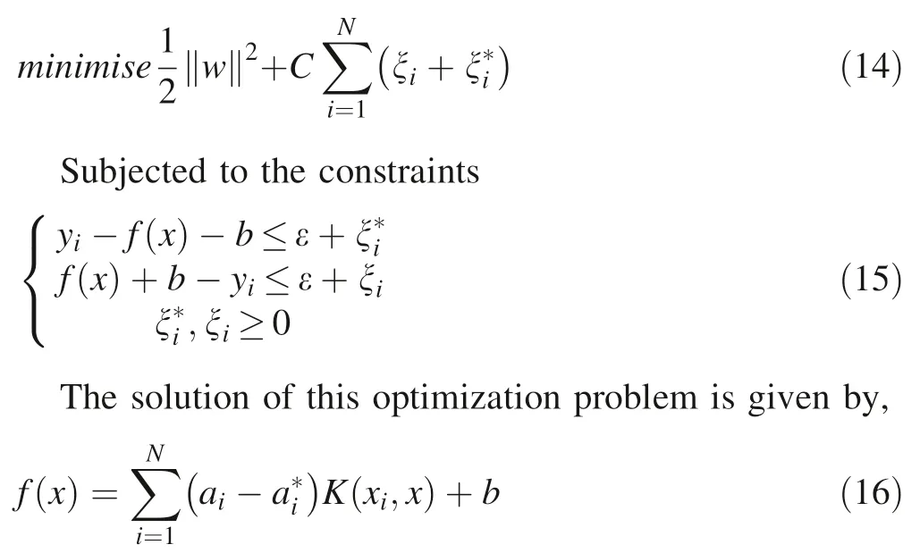
a
anda
are Lagrange multipliers andK
(x
,x
)is the kernel function(Herceg 2019).The performance of the SVM regression model is highly inf luenced by the type of the kernel function and setting the parameters C(capacity factor),ε(the error-insensitive zone)(Samui 2008).The commonly used kernel functions are linear,sigmoid,radial basis function and polynomial.In the current study,the kernel function and the different parameters are chosen by a trial and error method,where the kernel with high correlation coeff icient and least mean square error(MSE)results is used.
2.6 Data normalization
Normalization of data is common in artif icial intelligence modeling to prevent the models from domination by the large values(Ceryan 2014).Before running the modeling techniques,the inputs and outputs are normalized in the range 0–1 using the following equation.

X
is the normalized value,X
is the original value,X
andX
are the minimum and maximum of the original data,respectively.After modeling,the results are converted from the standard mode to the real values using the reverse equation as follows.

2.7 Evaluation and comparing model performance
The accuracy of the different modeling techniques(SK,SCOK,MLP-NN,and SVM)can be evaluated using different statistical measures through the f it of goodness approaches that describe the errors associated with the different models(Zounemat-kermani et al.2014).In this study,three common statistical parameters are used to evaluate the performance of the prediction models.The correlation coeff icient(R),which is def ined as the degree of the relationship between the observed and the predicted values,the root mean square error(RMSE),and the Mean absolute error(MAE)is expressed as follows:

3 Results and discussions
3.1 Input selection
The raw covariates are chosen using prior knowledge about the entire modeling problem,but the key covariates are selected using MLSR,which helps to exclude the covariates that do not have a signif icant effect on the modeling techniques.In this study,eight f ield measurement covariates(ECw,pH,Na%,SAR,cations+anions,clay%,sand%,and silt%)and eight environmental covariates(Elevation,aspect,curvature,slope,TWI,LST,NDVI,and SAVI)are candidates for inclusion in MLSR and predictors of ECs of the topsoil(TS)and the subsoil(SS).
Table 1 shows the results of applying MLSR procedure for the f ield measurement and the environmental covariates,including p values,variance inf lation factors(VIF),tolerance,unstandardized coeff icients(B),standardized coeff icients(),and the determination coeff icient(R).

Table 1 Results of the MLSR for the f ield measurement and environmental covariates
If aP
value is less than the threshold(α=0.05),the null hypothesis(i.e.,the covariates have no signif icant effect on the output variable,ECs)is rejected and the difference is statistically signif icant.On the other hand,if the P-value is greater thanα,the null hypothesis is conf irmed and there is no statistically signif icant difference.The tolerance and the variance inf lation factor(VIF)indices of the multicollinearity test are used to ensure the accuracy of MLSR results.The tolerance index indicates the percentage of variations in each covariate,which is not identif ied by other covariates.VIF=1 indicates that the covariate of interest does not correlate with the other covariates;1<VIF<5 shows moderate correlation and VIF>5 indicates a high correlation(Zounemat-kermani et al.2020).From the MLSR outputs,it is possible to see that the silt percentage with ECwand pHware the optimal combination of f ield covariates to predict ECs(TS)with a coeff icient R=0.599,while the optimal combination to predict ECs(SS)is sand percentage plus ECwwith R=0.706.For the environmental covariates,LST,TWI and elevation are the optimal predictors of the ECs of both depths,with R=0.620 and 0.530 for ECs(TS)and ECs(SS),respectively.The regression equations of ECs are as follows.

These optimal predictors of ECs(f ield measurement and environmental covariates)issued from MLSR are used as inputs for SCOK,MLP-NN,and SVM modeling techniques.
3.2 Descriptive statistics of the input and output data
3.2.1 Output data
The descriptive statistics of soil salinity of 136 samples from 68 sites(54 for training and 14 for testing)are summarized in Table 2.The soil salinity of the training dataset varied from 0.15 to 7.93 and 0.14 to 7.42 mS/cm for ECs(TS)and ECs(SS),respectively.The ECs of the testing dataset varied from 0.16 to 5.43 and 0.13 to 6.5 mS/cm for ECs(TS)and ECs(SS),respectively.The mean value of ECs takes values between the different depths,where the topsoil had the highest mean values.Furthermore,the mean value of ECs(TS)is higher than ECs(SS),with a mean value of 1.73 mS/cm.These results may be due to the accumulation of salt in the topsoil as a result of evaporation.The coeff icient of variation(CV)of ECs has values from 110%to 128%,which indicates a strong variation of salinity in the study area.This strong spatial variation of soil salinity may be due to the high variation of soil texture(slight textures in the eastern and heavy in the western part of the study area),land use,and irrigation schedules.
3.2.2 Input data
Table 3 summarizes the descriptive statistics of the f ield and the environmental covariates resulting from MLSR as the optimal predictors of ECs in the study area.The ECw varied from 1.13 to 12.01 mS/cm with a mean value of 4.23 mS/cm and a coeff icient of variation of 45.39%.In the study area the pH of groundwater(pHw)is neutral,which ranges from 7.19 to 7.84.The sand%of the topsoil and the subsoil have almost the same values with variations from 1.55%to 92.5%and 1.35%to 89.48%for the top soil and subsoil,respectively.The silt%is characterized by a high variation in the study area(CV=74.79%).The elevation of El Outaya plain varies between 173 m and 254 m.

Table 2 Descriptive statistics of ECs dataset used for training and testing
3.3 Geostatistical models
3.3.1 Simple kriging(SK)
In this study,SK is used for mapping the spatial distribution of soil salinity based only on the f ield measurements of ECs.The Kolmogorov and Smirnov test(KS test)revealed that the data of ECs for 54 training sites of both depths are not normally distributed;therefore,data are subjected to the normal score transformation.Fitting a theoretical semivariogram model to the empirical semivariogram is the main processing step in Kriging techniques.Different models are tried(Spherical,Gaussian,exponential…etc.)and the best f it is determined based on the cross-validation results(Lowest RMSE).
Figures 7a and b show the best semivariogram models selected for ECs(TS),ECs(SS),respectively and their different parameters.A spherical model with a nugget effect value of 0.051,the partial sill of 1.587,and a range of 32309 m is used for ECs(TS),while a Gaussian model with a nugget effect of 0.212,partial sill of 1.2,and a range of 26216 m is taken into consideration for ECs(SS).The nugget to sill ratio,which is used for the determination of the level of spatial dependence(Cambardella et al.1994),indicates a strong spatial dependence of soil salinity in both models.
The results of the performance criteria for training and testing stages are provided in Table 4.SK technique shows results that are more accurate in the testing stage.The MAE,RMSE,R are calculated respectively as 0.61,0.85,0.874 for ECs(TS),0.81,1.2,0.927 for ECs(SS).
The resultant maps of soil salinity from SK(Fig.8)show the spatial distribution of different soil salinity classes in the top and subsoils in El Outaya plain.The maps indicate approximately the same overall distribution of ECs classes in the study area.For the interpretation of the salinity level results,one can adopt the soil salinity classif ication of the Soil Test Handbook for Georgia(Abuelgasim and Ammad 2018),which is compatible with the analysis method employed in this paper for the measuring ECs(Table 6).
It is apparent from Fig.8 and Table 5,the dominance of two main salinity classes,the slightly saline to low salinity class and excessively high salinity class.The slightly saline/low salinity is located generally in the western part of the study area with area percentages of 41.14%,40.57%,for ECs(TS),ECs(SS),respectively.The excessively high salinity class is in the eastern part of the plain,where the agriculture is more intensive,with area percentages of 36.78%,37.70%for ECs(TS),ECs(SS),respectively.
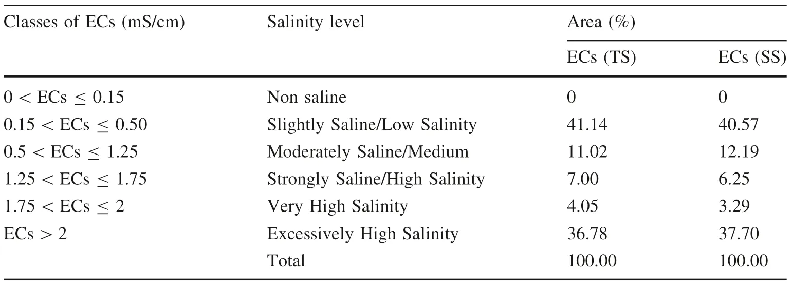
Table 5 The area percentages of different soil salinity classes of SK maps

Fig.8 Prediction maps of soil salinity using SK:a ECs(TS),b ECs(SS)
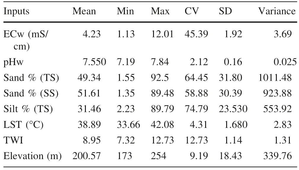
Table 3 Descriptive statistics of the input covariates

Table 4 Prediction performance measures of SK for training and testing datasets
The scatter plot of the measured soil EC and the estimated mean errors(Fig.9)using SK reveals an overestimation of the high ECs values and an underestimation of the low ECs value.This over-estimation can reach the maximum ECs(TS)and ECs(SS)values as equal to 3.4 and 3.7 mS/cm,respectively.On the other hand,the underestimation can have a maximum ECs(TS)value of 3.2 mS/cm and a minimum ECs(SS)value of 5.5 mS/cm.

Fig.7 Semivariograms and f itted models of a ECs(TS),b ECs(SS)

Fig.9 Scatter plots of measured soil EC and the estimated mean errors using SK:a ECs(TS),b ECs(SS)
3.3.2 Simple cokriging(SCOK)
3.3.2.1 SCOK with f ield covariates
Figure 10 shows the experimental auto semivariograms of ECs(TS),ECs(SS),and their f itted models.Their different cross semivariograms with the f ield covariates are shown in Fig.11.All the experimental and cross semivariograms are f itted with spherical models.The semivariogram model gives information about the autocorrelation of a spatial variable,while the cross covariogram provides information on cross correlation between two related spatial variables(Wang et al.2013).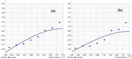
Fig.10 Auto semivariograms of ECs using f ield covariates:a ECs(TS),b ECs(SS)
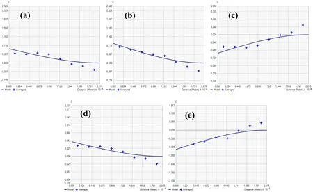
Fig.11 Cross covariograms between ECs and f ield covariates using SCOK:a ECs(TS)—ECw,b ECs(TS)—Silt(TS),c ECs(TS)—pHw,d ECs(SS)—ECw,e ECs(SS)—Sand(SS).All using spherical models
The parameters of the different semivariograms and cross covariograms are tabulated in Table 6.The models are f itted using different parameters(Nugget effect(C0),Sill(C),and ranges(a)).The nugget to sill ratios(C0/(C+C0))for all the auto semivarigram models of ECs indicate strong spatial dependences,with values of 5.68%and 14.04%for ECs(TS)and ECs(SS),respectively.The intrinsic factors are the main causes of strong dependence,while weak dependence is caused by extrinsic factors(Wang et al.2013).
3.3.2.2 SCOK with environmental covariates
Figures 12 and 13 show respectively the f itted auto semivariograms and cross covariograms models of ECs prediction using SCOK with the environmental covariates.ECs(SS)experimental variograms that are f itted using Gaussian models and ECs(TS)with a spherical model(the best model was chosen based on cross-validation results).Their different parameters are listed in Table 7.The nugget to sill ratio indicates strong spatial dependence for ECs(TS),with a value of 6.81%,and a moderate spatial dependence for ECs(SS)at a value of 25.20%.The MAE,RMSE,and R performance statistics of training and testing periods for SCOK with f ield covariates and SCOK with environmental covariates are given in Tables 8.All the models show accurate results in the testing period.For ECs1(SS),SCOK with ECw1 and sand(TS)covariates yield more accurate results than SCOK with LST1 and TWI covariates,with the smallest MAE of 0.44,RMSE of 0.59,and the highest R of 0.972 and,respectively.With MAE of 0.86,0.48 and 0.57;RMSE of 1.38,0.56 and 0.77;and R of 0.867,0.917 and 0.981,SCOK of ECs1(TS),ECs2(TS)and ECs2(SS)using LST2,TWI and elevation as covariates show more accurate results than SCOK using f ield covariates.

Table 6 Parameters of the auto semivariogram models for ECs and their cross covariogram models(using f ield covariates)

Fig.12 Auto semivariograms of ECs using environmental covariates:a ECs(TS),b ECs(SS)
3.3.3 Artif icial neural network and machine learning models
3.3.3.1 Multilayer
perceptron
neural network
(MLPNN)
Different MLP-NN models with Broyden–Fletcher–Goldfarb–Shanno(BFGS Quasi-Newton)back propagation algorithm are constructed for predicting soil salinity(ECs)in El Outaya plain using f ield covariates and environmental covariates as inputs.Tables 9 and 10 show the properties of the MLP-NN models for predicting ECs with f ield and environmental covariates,respectively.The optimal MLPNN structure,the number of hidden neurons and the activation functions are identif ied using a trial and error procedure by varying the number of hidden neurons from 1 to 20 and checking the performance criteria generated automatically by the software(the least SOS and highest R).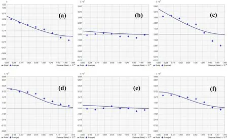
Fig.13 Cross covariograms between ECs and environmental covariates using SCOK:a ECs(TS)—LST,b ECs(TS)—TWI,c ECs(TS)—Elevation,d ECs(SS)—LST,e ECs(SS)—TWI,f ECs(SS)—elevation

Table 7 Parameters of the auto semivariogram models for ECs and their cross covariogram models(using environmental covariates)
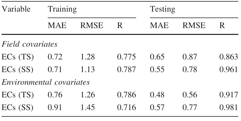
Table 8 Prediction performance measures of SCOK for training and testing datasets
As shown in Table 9,MLP(3-8-1)with logistic activation function in the hidden and output layers,and MLP(2-10-1)with Tanh hidden activation function and exponential output activation function are the best structures for predicting ECs(TS)and ECs(SS)using f ield covariates,respectively.The optimal structures of MLP-NN for predicting ECs(TS)and ECs(SS)are,respectively,MLP(3-5-1)with logistic function in the hidden layer and exponential activation function in the output layer,and MLP(3-5-1)with logistic activation function in both hidden and output layers.The selected structures show the lowest error values(SOS)during the training and testing stages compared to the other trained structures.
Table 10 shows the calculated performance criteria for the evaluation of MLP-NN models using f ield and environmental covariates.The performance criteria showed accurate results for training and testing periods with more accuracy in the testing stage.
From Table 10,MLP-NN modeling using f ield covariates as inputs show more accuracy in predicting ECs(SS)with MAE of 0.5 and 0.38,RMSE of 0.76 and 0.6,and R of 0.968 and 0.903 in the training and testing periods,respectively.For MLP-NN modeling environmental covariates as inputs,the MAE and RMSE performance criteria of the testing stage indicate more accurate results in predicting ECs(TS)than ECs(SS),with MAE of 0.43 and 0.95,RMSE of 0.6 and 1.22,and R of 0.946 and 0.961,respectively.

Inputs Output ANN structure Training error(SOS)Testing error(SOS)Hidden activation Output activation–n Field covariates ECw,silt(SS),pHw ECs2(TS) MLP 3-8-1 0.005 0.008 Logistic Logistic ECw,sand(SS) ECs2(SS) MLP 2-10-1 0.005 0.003 Tanh Expo Environmental covariates LST,TWI,elevation ECs2(TS) MLP 3-5-1 0.012 0.003 Logistic Expo LST,TWI,elevation ECs2(SS) MLP 3-5-1 0.012 0.014 Logistic Logistic
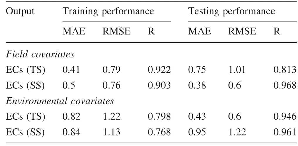
Table 10 Performance measures of MLP-NN models using environmental covariates

The results of SVM models’performance in terms of MAE,RMSE and R during the training and testing periods are presented in Table 12 from which SVM models for predicting ECs(SS)by using of ECw and sand percentage as inputs show clearly superior performance in the training and testing stages with MAE of 0.61 and 0.58,RMSE of 1.01 and 0.88,and R of 0.824 and 0.939,respectively.The calculated performance criteria of SVM modeling with environmental covariates indicate a superior performance for the prediction of ECs(TS)with the lowest MAE(0.69)and RMSE(0.93)during the testing period,while the correlation coeff icients are approximately the same(0.903 and 0.922).
4 Discussion and comparison of the different models
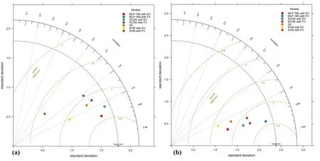
For the purpose of more clarity and a better comparison between the different modeling techniques,the Taylor diagram during the testing period was utilized(Fig.14).This diagram is a graphical framework that allows the comparison of different models at the same time and provides a concise statistical summary of how well patterns match each other in terms of their correlation,the ratio of their standard deviations,and their root-mean-square difference(Santos et al.2019;Koulla et al.2019).The overall comparisons between the different modeling techniques to predict the soil salinity in terms of ECs in El Outaya plain illustrate the superiority of MLP-NN over the other modeling methods,either by using the f ield covariates(ECs(SS))or the environmental covariates[ECs(TS)].
Taylor diagram(Fig.14)shows that MLP-NN using LST,TWI,and elevation as inputs is the best model to predict the topsoil salinity,where it could explain 90%of ECs(TS)variability in El Outaya plain and SVM using ECw,silt percentage,and pHw is the worst model with R=0.49.For the prediction of ECs(SS),the MLP-NN model,which used ECw and sand percentage as inputs provided better performance results than the other models and could explain 95.5%of the topsoil and the subsoil ECs variability in El Outaya plain.However,SCOK with the same covariates could explain 92.5%ECs(SS)variability in the study area.

Output Kernel function C εTraining errors(MSE) Testing Errors(MSE)Field covariates ECs(TS) RBF 0.3 0.1 0.2 0.046 0.043 ECs(SS) RBF 14 1.0 1.0 0.019 0.015 Environmental covariates ECs(TS) Polynomial 3.0 1.0 0.30 0.029 0.014 ECs(SS) Polynomial 4.0 0.10 0.33 0.031 0.041

Input combination Output Training Testing MAE RMSE R MAE RMSE R Field covariates ECw,pHw.Silt(TS) ECs(TS) 0.94 1.68 0.768 0.83 1.36 0.698 ECw,Sand(SS) ECs(SS) 0.61 1.01 0.824 0.58 0.88 0.939 Environmental covariates Elevation,LST,TWI ECs(TS) 0.86 1.33 0.818 0.69 0.93 0.903 Elevation,LST,TWI ECs(SS) 0.96 1.27 0.716 1.2 1.54 0.922
The developed models are the f irst for the prediction of soil salinity in our study area based on both environmental and f ield covariates.The selection of the proper inputs from all the raw parameters and the type of the adopted model are the main factors inf luencing the prediction performance of soil salinity,which can be improved by using very high-resolution satellite images(hyper-spectral images)and DEM as well as improving sampling method of groundwater and soil samples.
As mentioned above,the farmers of the study area are using high saline groundwater(high ECw)for irrigation,such practice has led to the destruction of soil texture and the soil salinity increase,which can be observed in the f ield by white crust on the soil surface.The accumulation of salts and development of soil salinity in the top and the subsoil are inf luenced by the proportion of soil particles,where the concentration of salts in soils increases with the decrease of the percentage of soil particles.Thus,the heavy soils(the eastern part of the study area)retain high amounts of salts.
An increase in the agricultural irrigation surface is important for the socio-economic development of the study area,but it was to the detriment of soil quality,which is largely affected by secondary salinization,the latter affects almost all the aspects of crop development and reduces yields.It is suggested to raise awareness among farmers about the dangers of saline water for irrigation and encourage them to apply appropriate leaching,drainage systems,desalination of groundwater by reverse osmosis,and fertigation using modern technologies to minimize soil damages due to secondary salinization.
5 Conclusion
The present study aimed to improve the prediction of top soil and sub soil salinity in El Outaya plain by using of two categories of covariates,the f ield covariates that affect directly the soil salinization(soil and water properties)and the environmental covariates(remote sensing and topographic covariates).Multiple linear stepwise regression,simple Kriging(SK),simple cokriking(SCOK),multilayer perceptron neural network(MLP-NN)and support vector machine(SMV)are employed for modeling purposes.The results show that the spatial prediction of soil salinity could be improved using cokriging with f ield and environmental auxiliary variables.Compared to SK,SCOK provides the lowest mean absolute errors(MAE)and root mean square errors(RMSE),and the highest correlations(R)between the measured and the predicted soil salinity.The spatial prediction maps of ECs indicated low concentrations in the western part of El Outaya plain,whereas the high concentrations located in the eastern part,where the agriculture is more intensive,the irrigation water is more saline and the soil is characterized by heavy textures.
The comparison of the performance of the different modeling techniques depicts the superiority of MLP-NN in the accuracy of estimating soil salinity with lower MAE and RMSE,and higher Pearson’s correlation coeff icients.The results of SCOK are close to those of MLP-NN.In addition,the combination of ECw and sand percentage from the f ield covariates and TWI,LST and elevation as inputs to MLP-NN and auxiliary variables to SCOK can estimate and improve the predictions of soil salinity in the study area.
Acknowledgement
s The corresponding author would like to thank Pr.Zekai S¸en of Medipol University(Turkey)for his thoughtful and insightful comments on draft versions of this paper.Compliance with ethical standards
Conf lict of interest
The authors declare that they have no conf lict of interest.- Acta Geochimica的其它文章
- Validating the deep time carbonate carbon isotope records:effect of benthic f lux on seaf loor carbonate
- Petrology and geochemical framework of dolerites dykes of Temte´,North Cameroon,Central Africa
- Interaction of Ca2+and soil humic acid characterized by a joint experimental platform of potentiometric titration,UV-visible spectroscopy,and f luorescence spectroscopy
- Trace and rare earth element geochemistry of the black and grey shales of the Calabar Flank,Southeastern Nigeria:constraints on the depositional environment and the degree of metal enrichment
- Geochronological and geochemical comparison of Precambrian meta-maf ic volcanics in Zhongtiaoshan and Lu¨liangshan Regions in Shanxi,North China Craton
- Mineralogy and geochemistry of sands of the lower course of the Sanaga River,Cameroon:implications for weathering,provenance,and tectonic setting

