Predicting Lung Cancers Using Epidemiological Data: A Generative-Discriminative Framework

Jinpeng Li, Member, IEEE, Yaling Tao, and Ting Cai

Abstract—Predictive models for assessing the risk of developing lung cancers can help identify high-risk individuals with the aim of recommending further screening and early intervention. To facilitate pre-hospital self-assessments, some studies have exploited predictive models trained on non-clinical data (e.g.,smoking status and family history). The performance of these models is limited due to not considering clinical data (e.g., blood test and medical imaging results). Deep learning has shown the potential in processing complex data that combine both clinical and non-clinical information. However, predicting lung cancers remains difficult due to the severe lack of positive samples among follow-ups. To tackle this problem, this paper presents a generative-discriminative framework for improving the ability of deep learning models to generalize. According to the proposed framework, two nonlinear generative models, one based on the generative adversarial network and another on the variational autoencoder, are used to synthesize auxiliary positive samples for the training set. Then, several discriminative models, including a deep neural network (DNN), are used to assess the lung cancer risk based on a comprehensive list of risk factors. The framework was evaluated on over 55 000 subjects questioned between January 2014 and December 2017, with 699 subjects being clinically diagnosed with lung cancer between January 2014 and August 2019. According to the results, the best performing predictive model built using the proposed framework was based on DNN. It achieved an average sensitivity of 76.54% and an area under the curve of 69.24% in distinguishing between the cases of lung cancer and normal cases on test sets.

I. INTRODUCTION

LUNG cancer is a major threat to humankind [1]. In China,the prevalence of lung cancer in men is 52 cases per 100 000 people, which makes it the first among all cancers. In women, the prevalence is 26.7 cases per 10 000 people, which makes it the second cancer following breast cancer, which leads at 30.4 cases per 100 000 people [2]. Since the current understanding of phenomena associated with lung cancer appearance and evolution is not sufficient for early detection,lung cancer is generally discovered late. As a result, the prognosis is poor [3]. More than 50% of cancers (including the lung cancer) could be prevented if the current knowledge of risk factors was utilized in risk assessments [4], [5].Therefore, moving medical interventions from treatment to prevention can potentially save lives [4], [6].

Identifying risk factors and making prediction rules for diseases have been used in clinical practice to assist decisionmaking and counseling [4], [7]. Using epidemiological questionnaires to collect risk factors and making predictions based on them is an economic and convenient approach to popularize disease prevention among the public. The Harvard cancer risk index (HCRI) research group developed the first comprehensive cancer risk assessment system and covered common cancers that accounted for 80% of all incidences in the United States [4], where lung cancer ranks the third among all cancers in terms of morbidity and mortality. On the basis of the HCRI, the Chinese National Cancer Center and Chinese Academy of Medical Sciences released the questionnaire on early diagnosis and treatment of urban cancer (EDTUC) in 2012. The questionnaire involves risk factors identified by experienced epidemiologists and clinical oncologist and is adjusted to suit Chinese people. Fig. 1 demonstrates that the questionnaire involves no clinical input to ensure the manageability of pre-hospital self-assessment. Risk factors are the foundation of the decision-making process on lung risk evaluation. The decision rules are based on the weighted summation of risk factors, where the weights are assigned according to expert opinions. This process brings subjectivity.This study considers clinical records (with lung cancer diagnoses) from January 2014 to August 2019 to build a deep learning lung cancer risk model (LCRM). The LCRM predicts risk scores indicating whether a person is under a high lung cancer risk. Our main contributions are listed as follows:

1) It is the first study on cancer prediction using EDTUC data covering the population of major cities in China. The study validates the effectiveness of risk factors and demonstrates the effectiveness of deep learning in predicting lung cancers based on non-clinical information.

2) The proposed model considers significantly more risk factors compared to existing methods.

3) The Wasserstein generative adversarial network(WGAN) is employed for auxiliary sample generation; it is shown to outperform the synthetic minority oversampling technique (SMOTE).

Fig. 1. The proposed data-driven lung cancer risk predictive model. The risk factors involve six aspects of epidemiological information.

4) The performance of the proposed method is validated in ablation experiments on real-life data.

II. RELATED WORK

Lung cancer is a common threat to human health. According to a survey in 2016, lung and bronchus cancers account for 14% of new cancer cases and 28% of cancer-related deaths in the United States [5]. In China, new cases and death rates from lung cancer rank the top two in both males and females[6]. The late diagnosis of lung cancer results in an increased death risk and a poor five-year survival rate of less than 20%[5]. Predicting lung cancer at an early stage helps identify high-risk population with the aim to recommend further screening (e.g., chest low-dose computed tomography (CT))and prompt lifestyle changes (e.g., quit smoking). Therefore,predicting the lung cancer risk is of great significance in reducing the lung cancer threat.

There are mainly two approaches to predicting lung cancer risks. The first approach is building an epidemiological plus clinical assessment model (ECAM) based on clinical measures such as blood tests [8], CT [9], and gene sequencing[10]. The second approach is building an epidemiological model (EM) based only on factors that are easy to access such as gender, age, and smoking history. The advantage of the ECAM over the EM is the consideration of clinical modalities that can potentially improve the prediction performance.However, the EM has the advantages of convenience and low cost. This study focuses on the EM to develop an effective and convenient risk prediction solution. Clinical measures are reserved for the second stage conducted on high-risk population identified by the EM. Such a two-stage mode allows to reduce the cost of screening.

As an early example of the EM, Bach et al. [11] used age,gender, smoking duration, smoking intensity, smoking quit time, and asbestos exposure as risk factors to predict lung cancer risk within one year. Spitz et al. [12] included environmental tobacco smoke, family history of cancer, dust exposure, prior respiratory disease and smoking history variables to build a multivariable logistic regression model that achieved a sensitivity of 70%. Cronin et al. [13] built a model based on smoking variables for predicting lung cancer risk for the future ten years rather than one year; the model achieved an accuracy of 72% for internal studies and 89% for external studies. We speculate that the accuracy would improve as the predictive window becomes longer; however,predictive window such as ten years is too long to be applied.Screening once in a long period of time would allow cancers to develop and progress, whereas screening annually or every three to five years is more appropriate for detecting cancers at their early stages. Therefore, constructing predictive models that evaluate five-year (or shorter) risk is more feasible. The applicability of the three aforementioned models is uncertain since the recruited subjects were current or former smokers, or had asbestos exposure history; therefore, the resulting model is not suitable for predicting lung cancer risk for people without smoking or asbestos exposure history.

Several studies have included extensive information such as medical history, family cancer history, and living conditions to predict risks among more general population. In 2011,Tammemagi et al. [14] used age, body mass index (BMI), Xray history, education level, smoking status, smoking duration, pack years, family lung cancer history, and chronic obstructive pulmonary disease history to build a model for predicting lung cancer risks within nine years. In 2013,Tammemagi’s model was modified to compute risks within six years [15]. In 2012, Hoggart et al. [16] identified age,smoking status, smoking start age, smoking duration, and number of cigarettes per day as risk factors to implement a one-year risk predictive model. The age of the population considered in Hoggart’s study was between 40 and 65, which was lower than that of the population recruited for the majority of existing studies. Hoggart’s model achieved an area under the curve (AUC) of 84% for smokers, whereas the performance on non-smokers was poor. In 2018, Hart et al.[17] built a lung cancer prediction model based on 13 risk factors among the general population that achieved an AUC of 86% on the test set. The considered risk factors included age,BMI, heart disease, physical exercise, gender, smoking status,emphysema, asthma, diabetes, stroke, hypertension, Hispanic ethnicity, and race.

While some studies have included all-round information other than smoking status, the risk factors considered in these studies are still limited. Hoggart’s model [16] includes five factors, Bach’s model [11] and Etzel’s model [18] include six factors, Cassidy’s model [19] includes eight factors,Tammemagi’s model [14] includes nine factors, and Spitz’s model [12] includes 12 factors. These studies adopted statistical analysis to quantify associations between each factor and diagnostic result, and applied logistic regression(LR) to predict lung cancer incidence. Statistical analysis lacks the consideration of the cooperation between risks factors during prediction, while LR cannot effectively model the nonlinear relationship between risk factors. Hence, more advanced techniques are required to accurately predict lung cancer.

III. MATERIALS AND METHODS

This study focuses on the data collected by the EDTUC project from the urban population of Ningbo, China,considering 84 factors. This number of factors is significantly higher than that considered in existing studies. The factors can be used to describe a broad range of cancers, thus allowing the unified analysis of various common cancers. The EDTUC project evaluates cancer risks according to diagnoses made by epidemiologists. Decisions are made by setting a threshold on the sum of risk factors; the risk is found to be high if the sum exceeds the threshold. This approach lacks objectivity since it is not result-oriented and does not use the information from real diagnostic data to formulate decision rules. From the perspective of data-driven modeling, learning a mapping function between risk factors and clinical diagnosis is a practical and objective approach to predicting lung cancer. To the best of our knowledge, there is no other study on the automatic prediction of lung cancer based in the EDTUC data.This study compares the performance of three discriminative models, namely, LR, support vector machine (SVM), and deep neural network (DNN). The models were trained to perform binary classification on the EDTUC samples and answer the question of whether a person would develop lung cancer within the next five years. Since the number of positive samples in this domain is significantly lower than that of negative samples, this study employs two generative models,namely, a WGAN and a variational autoencoder (VAE), to oversample positive samples.

A. Data Retrieval

The EDTUC project was launched in 2012 and carried out in major cities in China. Ningbo was one of them. Data were collected using an epidemiological questionnaire covering more than one hundred risk factors of common cancers(ethical approval 15-070/997 was granted by the Ethics Committee of the Chinese Academy of Medical Sciences).The participation was voluntary, and inclusion criteria included the following:

1) Ningbo citizen aged between 40 and 74;

2) No serious organ dysfunction or mental diseases.

The data were mainly contributed by community and regional central hospitals. The data from each questionnaire was entered by an employee. To ensure data quality, each questionnaire was checked by an independent person. Samples with missing information or obvious errors were discarded.The questionnaires collected across Ningbo were gathered in the Health Commission of Ningbo, China. This study considered all the questions included in the EDTUC questionnaire except those related to family history around common cancers other than lung cancers. We noticed that there were some logical repetitions in the original version of the questionnaire. To reduce the dimensionality of the data(which was thought to be beneficial for building accurate yet simple machine learning models), we reduced the number of considered questions while preserving all information. In total, 84 questions were selected for this study; they are listed in Appendix. Furthermore, 55 891 valid and unique responses collected between January 2014 and December 2017 were included in the study. The name and identity card number were used in combination as the key word to retrieve medical records from the NHC medical database. Among 55 891 respondents, 699 were diagnosed with lung cancer from January 2014 to August 2019. Table I shows the summary of the data.Since the class imbalance is severe, using the original data for training models would make the models tilt excessively toward negative predictions. Class balancing is an important step for obtaining reliable LCRMs [20]. Two advanced generative models were used in this study to synthesize auxiliary positive samples. Fig. 2 summarizes the proposed approach for predicting lung cancer. The LCRM is a discriminative model computing risk scores based on the risk factors. To alleviate the influence of class imbalance during training, we exploit WGAN and VAE to synthesize auxiliary samples. The optimization principles of the generative models are also illustrated in Fig. 2.

TABLE I SUMMARY OF THE RETRIEVED DATA FOR LUNG CANCER PREDICTION

B. Wasserstein Generative Adversarial Network

Generative adversarial networks (GANs) [21], [22] refer to a class of sophisticated generative models that are able to replicate real-world entities by approximating their underlying data distributions. This study employed a GAN to synthesize additional positive samples by augmenting existing positive samples.

The GAN scheme is inspired by the zero-sum game from game theory; its basic structure includes a generator (G) and a discriminator (D) (Fig. 2(c)). G is trained to capture the real data distribution so as to synthesize samples as real as possible from a noise variable z (that can follow a Gaussian, uniform,or any other distribution). D is trained to distinguish whether a sample comes from the real world or is synthesized by G. The two models compete with each other. When the Nash equilibrium is reached, D is able to distinguish between real and synthesized samples, and G learns the distribution of data[21]. The overall training goal of GANs can be formulated as

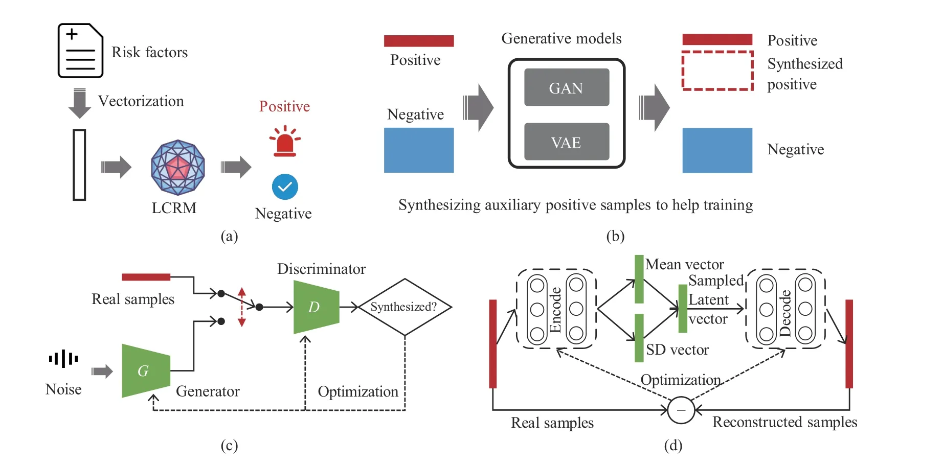
Fig. 2. The generative-discriminative framework for lung cancer risk prediction. (a) LCRM denotes a discriminative model automatically deciding whether to trigger an alar; (b) generative models synthesizing auxiliary samples to help training; (c) the training scheme of the GAN; (d) the training scheme of the VAE.

1) Sigmoid removal at the last layer of D;

2) No logarithm in the loss function of D;

3) Clipping D weights to a fixed small range (e.g.,[−0.1,0.1]) after each gradient update;

4) No momentum in the optimizer.

WGAN was used in this study to synthesize auxiliary positive samples and improve the training quality of LCRMs.

C. Variational Autoencoder

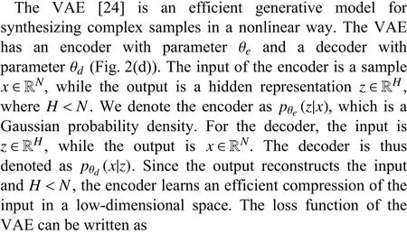
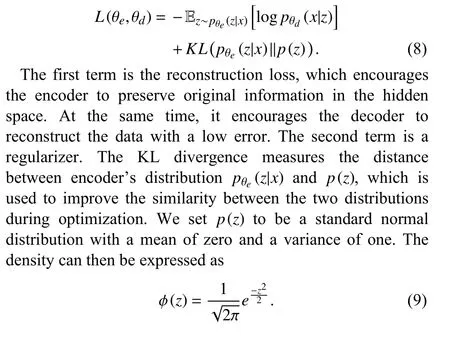
The regularizer makes the model meaningful by increasing the degree of similarity between similar data and degree of dissimilarity among different data in the hidden space. Since the hidden space is close to the normal distribution,meaningful samples can be synthesized by sampling from this distribution. A more detailed description of this process from the perspectives of probability theory can be found in [24] and[25]. In practice, when updating the model parameters, the mean and standard deviation of the encoder’s output are made close to those of the standard normal distribution. Once a model is trained, the decoder can be used to synthesize auxiliary positive samples by sampling the hidden space.

D. Lung Cancer Risk Model

The LCRM is a discriminative model, which computes the risk score on the basis of risk factors. Three machine learning models, namely LR, SVM, DNN, were used in this study to implement the LCRM. Their performance was compared in terms of the AUC, true positive rate (TPR or sensitivity), and true negative rate (TNR or specificity). The LR model feeds the output of a linear to a nonlinear sigmoid function to conduct binary classification; it is the most commonly-used machine learning method in relevant EM studies [5]. Unlike LR, SVM makes decisions based on boundary samples rather than all samples.

DNN learns the representations of data in a parameterintensive manner. The representations are learned using a hierarchical and end-to-end structure. Muhammad et al. [26]used a DNN to predict pancreatic cancer based on 18 features,demonstrating the effectiveness of this method.

E. Ablation Experiment Based on Risk Factors

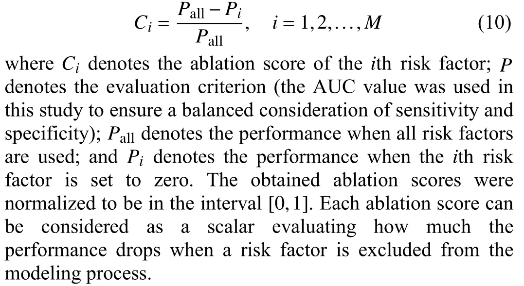
An LCRM makes predictions based on multiple risk factors.To quantitatively measure the contribution of each factor in the prediction process, we set the value of each risk factor value to zero one-by-one, retrained the model, and observed the result changes. For each risk factor, its ablation score was defined as

IV. ExPERIMENTS AND RESULTS

Only numeric values were accepted for open-text questions.One-hot encoding was used to represent answers for multiplechoice questions, resulting in a total of 148 features.

A. Baseline Models

To train baseline models, 699 negative samples were randomly selected from a total of 55 192 negative samples to match the number of available positive samples. A subset of 1 398 samples were thus obtained, which included an equivalent number of positive and negative samples. This dataset was split into training set (80%) and test set (20%). The values in each column of the training and test sets were normalized to be in the interval [0, 1].

The RBF kernel function was used for the SVM classifier;the class weights were set to be equal for positive and negative samples. Grid search with three-fold cross-validation was applied to find the c and gamma values that maximized the AUC value; the searching scope for both parameters was set to [2−3,23]. Table II summarizes the DNN structure; the number of layers and neurons was set experimentally for better performance. L2-regularizer (0.01) was applied to the second and third layers to avoid overfitting. The optimizer was set to Adam [27] with default parameters. The batch size was set to 32, the validation split during training was set to 20%, and the number of training epochs was set to 1000. Early stopping was applied with a patience of 10. The SVM and LR models were implemented using the Scikit-learn library [28],while the DNN model was implemented using the TensorFlow library.

TABLE II SUMMARY OF THE MODEL ARCHITECTURES

Table III shows the performance of the baseline models. It can be noticed from the table that the baseline models achieved similar and reasonable results when no clinical measures were used. In particular, the AUCs for the LR,SVM, and DNN models were 64.21%, 64.83%, and 64.91%,respectively.

B. Synthesizing Auxiliary Samples

To balance the classes, positive samples were first used to train the WGAN and VAE and synthesize auxiliary positive samples. This approach was compared to SMOTE.

The dimensionality of noise variable z in WGAN was 16;this noise variable follows a normal distribution. The details of the generator G and discriminator D are summarized in Table II. In particular, the clip value was set to 0.1, which means that the weights of D were clipped below 0.1. Since D is responsible for providing reliable gradients, its parameters are updated five times in each iteration before updating G parameters. As suggested in [22], the non-momentum optimizer RMSProp with a small learning rate of 0.0005 was used to search for solutions. The VAE details are also summarized in Table II. In particular, the Adam optimizer with default parameters was used to optimize VAE. Both WGAN and VAE were implemented using the Keras library running on top of TensorFlow.

TABLE III COMPARISON OF DIFFERENT OVERSAMPLING AND CLASSIFICATION METHODS

Fig. 3(a) demonstrates the impact of the number of synthesized samples on the DNN performance. In the figure,results are averages over five runs. In each run, the 699 positive samples were split into 560 training and 139 test samples. The positive augmentation fold (PAF) represents the number of times positive samples were augmented. For example, PAF=1 means that no synthesized samples were used during training. After the number of positive samples was determined, the same number of negative samples was randomly selected for training. According to the results,WGAN is superior to VAE and SMOTE. When PAF grows from one to two, the AUC increases for all the three methods.However, a higher number of synthesized samples does not always bring better results; the curves of the three methods all show fluctuations when PAF grows from three to ten. This phenomenon indicates that a large number of repetitive(similar) patterns may result in overfitting. Setting PAF to two yielded good performance with the minimal sample size on the considered dataset.

Several studies have suggested that making the numbers of positive and negative samples strictly equal is not necessary the best modeling approach [29]. To assess the impact of the number of negative samples on the model performance, the mean AUC of DNN was evaluated under different numbers of negative samples with PAF=2. The negative sampling fold( NS F) was used to represent the number of negative samples selected for training (Fig. 3(b)). For example, NS F=1 means that an equal number of negative and positive samples were used to train the model. For all the three oversampling methods, the optimal AUCs were achieved when NS F=1,although the results were similar when NS F=2. When NS F>4, the values of the AUC dropped significantly since optimization was dominated by the negative class. These empirical results suggest making a balanced training set.

Table III shows the results of different oversampling and classification methods ( PAF=2 , NS F=1). Oversampling methods have the potential of synthesizing noisy samples;hence two data cleaning methods were applied after oversampling:

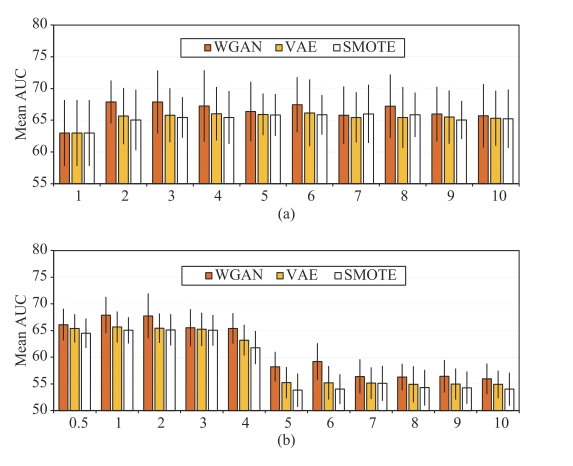
Fig. 3. Mean area under the curves (AUCs) of DNN impacted by (a) positive augmentation fold (PAF) and (b) negative sampling fold (NSF). PAF denotes the number of folds of synthesized positive samples. NSF denotes the number of folds of negative samples sampled with respect to the number of positive samples.

1) Edited Nearest Neighbors (ENN): For a synthesized positive sample, if the majority of its neighbors are negative samples, it is identified as a noisy sample and therefore is removed.

2) Tomek Link: For a sample A, if its nearest neighbor B comes from the opposite class, and the nearest neighbor of B is A, then the two samples have a Tomek link. Synthesized Tomek samples in the positive class were removed.

Data cleaning was performed using the imblearn library[30]. The Euclidean distance was used as the metric. The default setting was adopted for ENN (three neighbors).According to the mean AUCs on the test set, the impact of data cleaning on the model performance was unclear; no significant differences could be captured. Therefore, auxiliary samples synthesized by SMOTE, VAE, and WGAN had reliable class properties.

C. Comparisons With the State-of-the-Art Algorithms

We compare the proposed method with state-of-the-art outlier detection algorithms, undersampling algorithms and generative models. The results are summarized in Table IV.The generative adversarial active learning (GAAL) [31] has two versions: the single-objective GAAL (SO-GAAL) and the multi-objective GAAL (MO-GAAL). SO-GAAL uses a generator to synthesize minority data, and a discriminator to distinguish the minority data and the synthesized minority data. After reaching the Nash equilibrium, the discriminator is used as the outlier detector. MO-GAAL uses more generators to learn reasonable reference distributions of the dataset. The configurations of the generator and discriminator are consistent with that shown in Table II except that the activation function of the output layer of the discriminator is replaced by Sigmoid. We set the training epoch as 1 K. We apply the stochastic gradient descent with a momentum of 0.9 to optimize the generator (learning rate: 0.0001) and the discriminator (learning rate: 0.001). For MO-GAAL, we use 10 generators to conduct the experiment. The nearest sample of cluster center (NSCC) [32] is an effective undersampling method, which performs K-means clustering in the majority class, and the nearest sample of each center is regarded as minority samples. The EhrGAN [33] uses GAN to synthesize the electronic health records to enhance training. We adopt the GAN structure and learning configuration of the SO-GAAL to conduct the experiment. The symbol “*” is used to indicate statistically significant improvement (p < 0.05 according to the paired t-test) of the model with respect to the baseline.According to the results, the performance of VAE is basically the same as those of NSCC and EhrGAN. The WGAN we apply achieves the highest sensitivity (76.54%), specificity(71.08%) and AUC (69.24%) among all the methods.

TABLE IV COMPARISON WITH STATE-OF-THE-ART METHODS

D. Ablation Test Results for Risk Factors

Ablation tests were conducted to evaluate the effectiveness of each risk factor by evaluating the AUC drop when disabling each risk factor to a constant (zero) in turn. The computing criterion was set according to (10). The results were scaled to [0,1]. Fig. 4 shows the mean ablation score of each risk factor. The list of risk factors appearing on the horizontal axis can be found in Table V in Appendix. When different risk factors were disabled, the changes in the prediction results showed significant differences. The factors played different roles in modeling. While some factors impacted the result directly, others impacted it in a cooperatively coupled manner.

V. DISCUSSION

The best value of the AUC obtained on the test set was 69.24%, with a sensitivity of 76.54% and a specificity of 71.08%. Many lung cancer prediction models have been proposed in the literature based on different risk factors and target populations. Some studies have reported results obtained on entire datasets, without splitting them into training and test sets. This is the case with the Tammemagi’s model [14], for example, which achieved an AUC of 77%when considering nine risk factors. Those studies evaluating their models on separate test sets, have reported lower AUC scores. For example, Spitz’s model [12] built using 12 risk factors achieved AUCs for those who never smoked, were former smokers, and current smokers of 57%, 63%, and 58%,respectively. Etzel’s model [18] built using six risk factors achieved an AUC of 63%. Cassidy model [19] built using eight risk factors to predict lung cancer achieved an AUC of 70%. Cassidy’s model was built using 579 lung cancer cases,which is similar to the number of cases used to build the model proposed in this paper (699). Both models were built to predict five-year risk among general population. While the AUC score of Cassidy’s model is slightly higher than that of the model proposed in this paper (by 2.11%), the latter is tailored to the lifestyle of Chinese people, and therefore, still has a reference value.

This study employed VAE and WGAN for oversampling,and compared them with commonly-used SMOTE. When used in combination with the LR model, SMOTE, VAE, and WGAN allowed to achieve AUCs of 64.95%, 66.14%, and 66.99%, respectively. When used in combination with the DNN model, SMOTE, VAE, and WGAN allowed to achieve AUCs of 65.54%, 65.82%, and 69.24%, respectively. In both cases, the WGAN-based oversampling allowed to achieve the best AUC, sensitivity, and specificity. When combined with DNN, the advantage of WGAN is more significant (WGAN to VAE: p < 0.01; WGAN to SMOTE: p < 0.01; both evaluated using the paired t-test). At present, the main method to solve the problem of class imbalance is SMOTE. However, SMOTE is based on the linear interpolation and insufficient in synthesizing high-quality samples with high dimensions.Considering that the number of variables included in this study is more than previous studies, we propose to use two sophisticated nonlinear generative models, i.e., WGAN and VAE to generate samples in high-dimensional manifolds. The results validate the superiority of these methods. As nonlinear generative models, WGAN and VAE can be used in upsampling high-dimensional and complex data.

While SMOTE, VAE, and WGAN bring significant performance improvements, the unlimited oversampling of positive class does not bring continuous improvement. The experimental results in Fig. 3 confirm this viewpoint. In this study, the number of positive samples was significantly lower than that of negative samples. Oversampling may result in repetitive or similar positive patterns; this can provide a good performance on the training set but not the test set. In other words, models can become overfitted when an excessive number of synthesized samples are used for their training.

Fig. 4. Ablation test results demonstrating the impact of the considered risk factors. The ablation scores were computed according to (10). The results are represented as means over five runs. The error bars represent the standard deviation.

Compared to the LR and SVM models, the DNN model is more parameter-intensive. While this characteristic endows DNN with a strong fitting ability, it requires more training samples to search for parameters. Therefore, the performances of DNN, LR, and SVM are pretty much the same in the baseline. However, when synthesized samples are used to assist training, the performance of DNN is better than that of LR. We believe that DNN can outperform LR even further when more positive samples are included in the training set.

The presented ablation test demonstrates the relative contribution of each risk factor in the data-driven modeling.

1) Basic Information: Removing A02: Age leads to the largest performance decline. The possibility of developing lung cancer rises rapidly with age, as has been demonstrated elsewhere [34]. The elderly should pay more attention to lung cancer prevention. A01: Gender has a high ablation score.This is not surprising; the prevalence of lung cancer among Chinese men is about twice that among Chinese women [2].

2) Diet Habits: B01: Fresh vegetable is associated with lung cancer, which is consistent with a cohort study conducted among Chinese people [35], although the reasons have been less investigated. High ablation scores are also found for B07:Salt, B03: Meat, and B09: Pickled food. While B07 has not appeared in the literature, B03 and B07 have been investigated elsewhere. In particular, some recent studies have found convincing associations between large intake of red meat and lung cancer [36]. While some studies have investigated the associations between B09: Pickled food and lung cancer in China, no positive results have been found [37]. A recent study suggests that consuming pickled foods is associated with smoking and alcohol drinking, and the risk of lung cancer increases when these risk factors are present [38].

3) Living Conditions: Risk factors with high ablation scores include C04: Lampblack, C05: Smoking, C07: Total smoking years, and C09: Regular inhalation of secondhand smoke. All of these factors except for C04: Lampblack are associated with smoking. Both active smoking [39] and passive smoking[40] have been proved to be correlated with lung cancer in many studies. Stopping smoking is important for reducing the risk of lung cancer.

4) Psychology and Emotion: These factors have been relatively neglected in the literature. The ablation test results show that these “internal factors” are also important.

5) Medical History: High ablation scores are found for E05:Chronic bronchitis, E15: Duodenal ulcer, and E31:Hypertension. While E05: Chronic bronchitis has been proved to be associated with lung cancer [41], the other two factors require further investigation.

6) Family Cancer History: F07: Grandparents-in-law and F09: Mother’s brother or sister have relatively high ablation scores. These findings should be confirmed with more rigorous and large-scale epidemiological studies.

VI. CONCLUSION

The EDTUC questionnaire provides comprehensive information to facilitate lung cancer risk prediction. The LCRM learns decision rules automatically based on the clinical diagnosis in a data-driven manner, which avoids the subjectivity of human experience. In application, LCRM helps identify peoples with high risk of developing lung cancer within around five years. Further screenings and individualized interventions should be carried out to prevent lung cancer. The development of machine learning will help to improve the prevention-oriented medical system, so as to improve the human well-being.

The main limitation of this study is the focus on employing deep learning for lung cancer prediction, without considering the medical, biological, and oncological perspective.

As part of our future work, we plan to regularly update the LCRM as more data will be collected. We intend to package the model as software and combine its predictions with medical expertise using Bayes reasoning. Expert experience can help improve the interpretability of the LCRM and encourage its better performance when examples of positive cases are limited. In addition, the LCPM model can take clinical test variables, imaging data, and genetic data into consideration, so as to improve the prediction performance and have a prognostic evaluation function.

APPENDIX

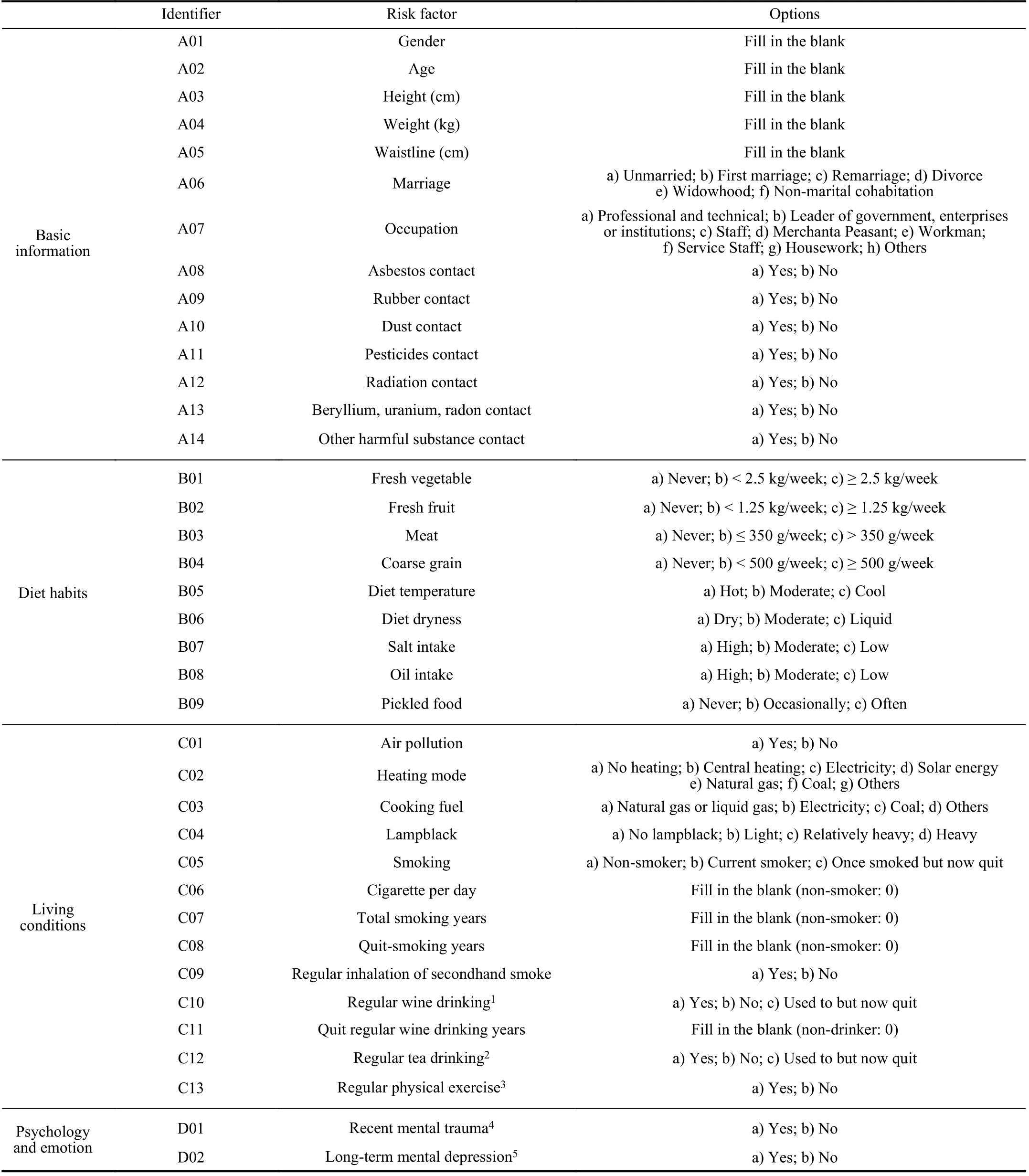
TABLE V RISK FACTORS OF LUNG CANCER PREDICTION

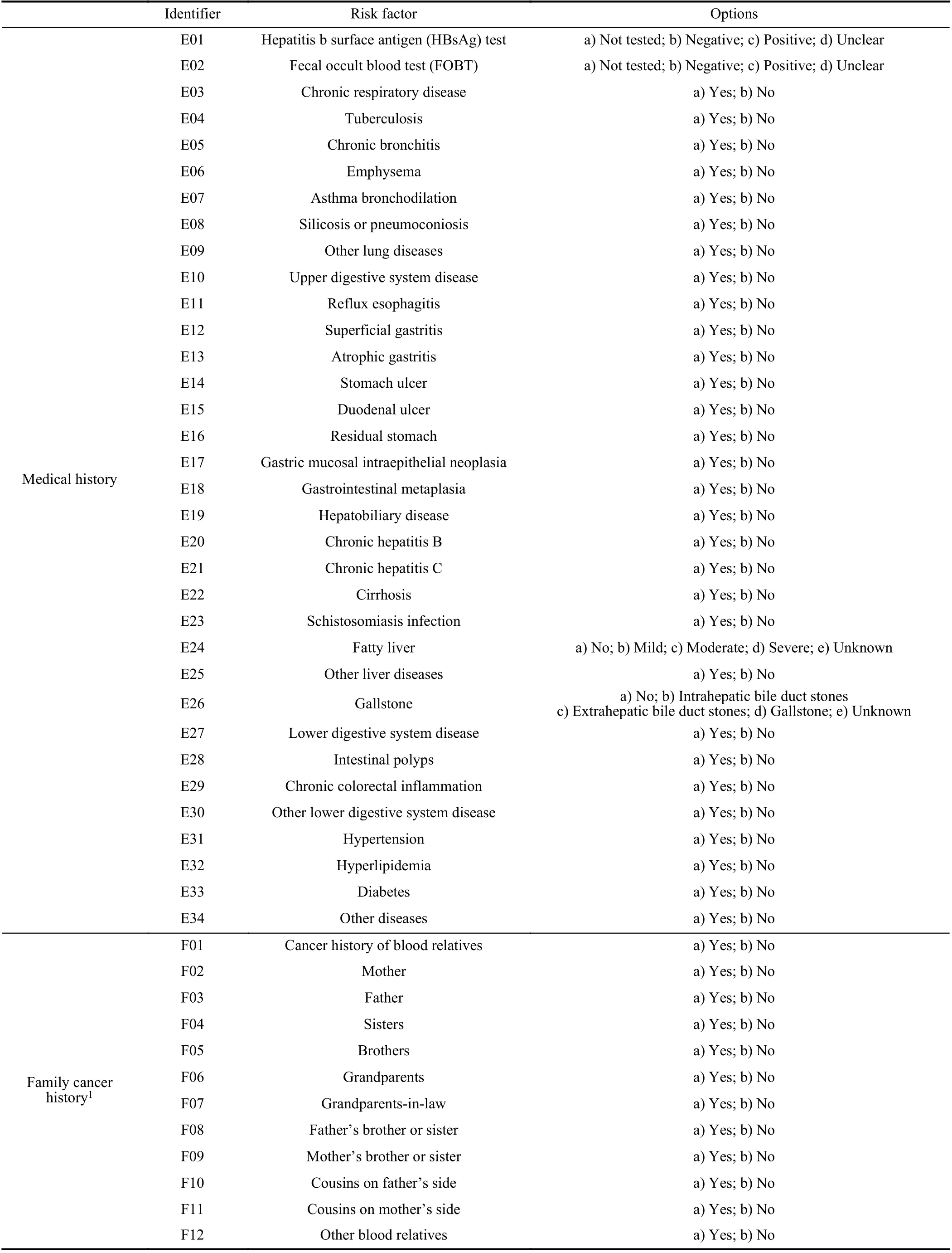
TABLE V(CONTINUED)

ACKNOwLEDGMENT

The authors would like to thank the Health Commission of Ningbo (HCN), China for providing questionnaire data, as well as providing clinical diagnosis records of lung cancer.