Causal Inference†

Kun Kuan*, Lan L, Z Gn, L Xu, Kun Zan, Bsu Lao, Huaxn Huan,Pn Dn, Wan Mao, Zao Jan

a College of Computer Science and Technology, Zhejiang University, Hangzhou 310058, China

b Department of Computer Science and Technology, Hefei University of Technology, Hefei 230009, China

c School of Mathematical Science, Peking University, Beijing 100871, China

d Department of Computer Science and Engineering, Shanghai Jiao Tong University, Shanghai 200240, China

e Department of Philosophy, Carnegie Mellon University, Pittsburgh, PA 15213, USA

f School of Humanities, Zhejiang University, Hangzhou 310058, China

g University of California Berkeley, Berkeley, CA 94720, USA

h Guanghua School of Management, Peking University, Beijing 100871, China

i Department of Government & Department of Statistics, Harvard University, Cambridge, MA 02138, USA

Keywords:Causal inference Instructive variables Negative control Causal reasoning and explanation Causal discovery Counterfactual inference Treatment effect estimation

A B S T R A C T Causal inference is a powerful modeling tool for explanatory analysis, which might enable current machine learning to become explainable. How to marry causal inference with machine learning to develop explainable artificial intelligence (XAI) algorithms is one of key steps toward to the artificial intelligence 2.0. With the aim of bringing knowledge of causal inference to scholars of machine learning and artificial intelligence, we invited researchers working on causal inference to write this survey from different aspects of causal inference. This survey includes the following sections: ‘‘Estimating average treatment effect: A brief review and beyond” from Dr. Kun Kuang, ‘‘Attribution problems in counterfactual inference”from Prof.Lian Li,‘‘The Yule-Simpson paradox and the surrogate paradox” from Prof.Zhi Geng, ‘‘Causal potential theory” from Prof. Lei Xu, ‘‘Discovering causal information from observational data” from Prof. Kun Zhang, ‘‘Formal argumentation in causal reasoning and explanation” from Profs.Beishui Liao and Huaxin Huang, ‘‘Causal inference with complex experiments” from Prof. Peng Ding,‘‘Instrumental variables and negative controls for observational studies” from Prof. Wang Miao, and‘‘Causal inference with interference” from Dr. Zhichao Jiang.

1. Estimating average treatment effect: A brief review and beyond

Machine learning methods have demonstrated great success in many fields, but most lack interpretability. Causal inference is a powerful modeling tool for explanatory analysis, which might enable current machine learning to make explainable prediction.In this article, we review two classical estimators for estimating causal effect, and discuss the remaining challenges in practice.Moreover,we present a possible way to develop explainable artificial intelligence (XAI) algorithms by marrying causal inference with machine learning.

1.1. The setup

1.2. Two estimators

Here, we briefly introduce two of the most promising estimators for treatment effect estimation and discuss them for the case with many observed variables.

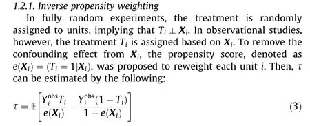
By combining propensity weighting and regression, it is also possible to estimate the treatment effect with a doubly robust method [2]. In high-dimensional settings, not all observed variables are confounders. To address this issue, Kuang et al. [3] suggest separating all observed variables into two parts: the confounders for propensity score estimation, and the adjustment variables for reducing the variance of the estimated causal effect.

1.2.2. Confounder balancing

In high-dimensional settings, different confounders can contribute to different confounding biases. Thus, Kuang et al. [5] suggest jointly learning confounder weights for confounders differentiation, learning sample weights for confounder balancing,and simultaneously estimating the treatment effect with a Differentiated Confounder Balancing (DCB) algorithm.

1.3. Remaining challenges

There are now more promising methods available for estimating treatment effect in observational studies, but many challenges remain in making these methods become useful in practice. Here are some of the remaining challenges:

1.3.1. From binary to continuous

The leading estimators are designed for estimating the treatment effect of a binary variable and achieve good performance in practice. In many real applications, however, we care not only about the cause effect of a treatment, but also about the dose response functions, where the treatment dose may take on a continuum of values.

1.3.2. Interaction of treatments

In practice, the treatment can consist of multiple variables and their interactions.In social marketing,the combined causal effects of different advertising strategies may be of interest.More work is needed on the causal analyses of treatment combination.

1.3.3. Unobserved confounders

The existence of unobserved confounders is equivalent to violation of the unconfoundedness assumption and is not testable.Controlling high-dimensional variables may make unconfoundedness more plausible but poses new challenges to propensity score estimation and confounder balancing.

1.3.4. Limited on overlap

Although the overlap assumption is testable, it raises several issues in practice, including how to detect a lack of overlap in the covariate distributions,and how to deal with such a lack,especially in high-dimensional settings.Moreover,estimating the treatment effect is only possible for the region of overlap.

Recently, related works have been proposed to address the above challenges, including continuous treatment [6], the interaction of treatments [7], unobserved confounders [8], and the limits on overlap [9,10].

1.4. Toward causal and stable prediction

The lack of interpretability of most predictive algorithms makes them less attractive in many real applications, especially those requiring decision-making.Moreover,most current machine learning algorithms are correlation based, leading to instability of their performance across testing data, whose distribution might be different from that of the training data. Therefore, it can be useful to develop predictive algorithms that are interpretable for users and stable to the distribution shift from unknown testing data.

By assuming that the causal knowledge is invariant across datasets, a reasonable way to solve this problem is to explore causal knowledge for causal and stable prediction. Inspired by the confounder-balancing techniques from the literature of causal inference, Kuang et al. [11] propose a possible solution for causal and stable prediction. They propose a global variable balancing regularizer to isolate the effect of each individual variable, thus recovering the causation between each variable and response variable for stable prediction across unknown datasets.

Overall, how to deeply marry causal inference with machine learning to develop XAI algorithms is one of key steps toward to the artificial intelligence(AI)2.0[12,13],and remains many special issues, challenges and opportunities.

2. Attribution problems in counterfactual inference

In this section, the input variable X and the outcome variable Y are both binary.

Counterfactual inference is an important part of causal inference. Briefly speaking, counterfactual inference is to determine the probability that the event y would not have occurred (y = 0)had the event x not occurred (x = 0), given the fact that event x did occur(x=1)and event y did happen(y=1),which can be represented as the following equation:

where yx=0is a counterfactual notion,which denotes the value of y when the setting is x=0 and the fixing effects of other variables are unchanged, so it is different from the conditional probability P （y |x=0）. This formula reflects the probability that event y will not occur if event x does not occur; that is, it reflects the necessity of the causality of x and y.In social science or logical science,this is called the attribution problem.It is also known as the‘‘but-for”criterion in jurisprudence. The attribution problem has a long history of being studied; however, previous methods used to address this problem have mostly been case studies, statistical analysis, experimental design, and so forth; one example is the influential INUS theory put forward by the Australian philosopher Mackie in the 1960s [14]. These methods are basically qualitative, relying on experience and intuition.With the emergence of big data,however,data-driven quantitative study has been developed for the attribution problem, making the inference process more scientific and reasonable.

Attribution has a twin problem,which is to determine the probability that the event y would have occurred(y=1)had the event x occurred(x=1),given that event x did not occur(x=0)and event y did not happen (y = 0). Eq. (7) represents this probability.

This equation reflects the probability that event x causes event y; that is, it reflects the sufficiency of the causality of x and y.

Counterfactual inference corresponds to human introspection,which is a key feature of human intelligence.Inference allows people to predict the outcome of performing a certain action, while introspection allows people to rethink how they could have improved the outcome, given the known effect of the action.Although introspection cannot change the existing de facto situation, it can be used to correct future actions. Introspection is a mathematical model that uses past knowledge to guide future action. Unless it possesses the ability of introspection,intelligence cannot be called true intelligence.

Introspection is also important in daily life. For example, suppose Ms. Jones and Mrs. Smith both had cancer surgery. Ms. Jones also had irradiation. Eventually, both recovered. Then Ms. Jones rethought whether she would have recovered had she not taken the irradiation. Obviously, we cannot infer that Ms. Jones would have recovered had she not take the irradiation, based on the fact that Mrs. Smith recovered without irradiation.

There is an enormous amount of this kind of problem in medical disputes, court trials, and so forth. What we are concerned with is what the real causality is, once a fact has occurred for a specific individual case. In these situations, general statistics data—such as the recovery rate with irradiation—cannot provide the explanation. Calculating the necessity of causality by means of introspection and attribution inference plays a key role in these areas [14].

As yet,no general calculation method exists for Eq.(6).In cases that involve solving a practical problem, researchers introduce a monotonic assumption that can be satisfied in most cases;that is:

The intuition of monotonicity is that the effect y of taking an action (x = 1) will not be worse than that of not taking the action(x=0).For example,in epidemiology,the intuition of monotonicity is not true for people who are contrarily infected(y=0)after being quarantined (x = 1), and who were uninfected(y = 1) before being quarantined (x = 0). Because of the monotonicity, Eq. (6) can be rewritten as follows:

In order to explain the relationship between the attributable risk fraction and the confounding factor,and their roles in the attribution problem (i.e., the necessity of causality) more specifically,we applied the example in Ref. [15]. In this example, Mr. A goes to buy a drug to relieve his pain and dies after taking the drug.The plaintiff files a lawsuit to ask the manufacturer to take responsibility. The manufacturer and plaintiff provide the drug test results(i.e.,experimental data)and survey results(i.e.,nonexperimental data),respectively.The data is illustrated in Table 1,where x = 1 denotes taking drugs, while y = 1 denotes death.

The manufacturer’s data comes from strict drug safety experiments, while the plaintiff’s data comes from surveys among patients taking drugs by their own volition. The manufacturer claims that the drug was approved based on the drug distribution regulations.Although it causes a minor increase in death rate(from 0.014 to 0.016),this increase is acceptable compared with the analgesic effect.Based on the traditional calculation of the attributable risk fraction (excess risk ratio), the responsibility taken by the manufacturer is

The plaintiff argues that the drug test was conducted under experimental protocols, the subjects were chosen randomly, and the subjects did not take the drug of their own volition.Therefore,there is bias in the experiment,and the experimental setting differs from the actual situation. There is a huge difference between observational data and experimental data. Given the fact of the death of Mr.A,the calculation of the manufacturer’s responsibility should obey the counterfactual equation. The result is

Therefore, the manufacturer should take full responsibility for the death of Mr. A.

Table 1 Experimental and non-experimental data for the example of a drug lawsuit.

In data science, there are simulated data and objective data,with the latter containing experimental data and observational data. Although observational data are objective, easily available,and low in cost, the confounding problems among them become an obstacle for causal inference [17]. In particular, there may be unknown variables (i.e., hidden variables) in an objective world.These variables are not observed, but may have effects on known variables—that is, the known variables should be sensitive to unmeasured confounding due to unknown variables.In this aspect,current studies on confounding are still in their infancy. Readers can refer to Ref. [18] for more detail.

3. The Yule-Simpson paradox and the surrogate paradox

An association measurement between two variables may be dramatically changed from positive to negative by omitting a third variable, Z; this is called the Yule-Simpson paradox [19,20]. The third variable, Z, is called a confounder. A numerical example is shown in Table 2.The risk difference(RD)is the difference between the proportion of lung cancer in the smoking group and that in the no-smoking group, RD = (80/200) - (100/200) = -0.10, which is negative. If the 400 persons listed in Table 2 are split into males and females, however, a dramatic change can be seen (Table 3).The RDs for both males and females are positive, at 0.10. This means that while smoking is bad for both males and females,separately, smoking is good for all of these persons.

The main difference between causal inference and other forms of statistical inference is whether the confounding bias induced by the confounder is considered. For experimental studies, it is possible to determine which variables affect the treatment or exposure; this is particularly true for a randomized experiment,in which the treatment or exposure is randomly assigned to individuals, as there is no confounder affecting the treatment. Thus,randomized experiments are the gold standard for causal inference. For observational studies, it is key to observe a sufficient set of confounders or an instrumental variable that is independent of all confounders. However, neither a sufficient confounder set nor an instrumental variable can be verified by observational data without manipulations.

In scientific studies, a surrogate variable (e.g., a biomarker) is often measured instead of an endpoint, due to its infeasible measurement; and, then, the causal effect of a treatment on theunmeasured endpoint is predicted by the effect on the surrogate.The surrogate paradox means that the treatment has a positive effect on the surrogate, and the surrogate has a positive effect on the endpoint, but the treatment may have a negative effect on the endpoint [21]. Numerical examples are given in Refs. [21,22].This paradox also queries whether scientific knowledge is useful for policy analysis[23].As a real example,doctors have the knowledge that an irregular heartbeat is a risk factor for sudden death.Several therapies can correct irregular heartbeats, but they increase mortality [24].

Table 2 Smoking and lung cancer.

Table 3 Smoking and lung cancer with populations stratified by gender.

Yule-Simpson paradox and the surrogate paradox warn about that a conclusion obtained from data can be inverted due to unobserved confounders and emphasize the importance of using appropriate approaches to obtain data. To avoid the Yule-Simpson paradox, first, randomization is the golden standard approach for causal inference. Second, the use of an experimental approach to obtain data is expected, if randomization is prohibited, as such an approach attempts to balance all possible unobserved confounders between the two groups to be compared. Third, an encouragement-based experimental approach—in which benefits are randomly assigned to a portion of the involved persons, such that the assignment can change the probability of their exposure—can be used to design an instrumental variable. Finally, for a pure observational approach,it is necessary to verify the assumptions required for causal inference using field knowledge, and to further execute a sensitivity analysis for violations of these assumptions. The two paradoxes also point out that a syllogism and transitive reasoning may not be applicable to statistical results. Statistically speaking, smoking is good for both males and females, and the studied population consists of these males and females; however, the statistics indicate that smoking is bad for the population as a whole.Statistics may show that a new drug can correct irregular heartbeats, and it is known that a regular heartbeat can promote survival time, both statistically speaking and for individuals; however, the new drug may still shorten the survival time of these persons in terms of statistics.

4. Causal potential theory

Extensive efforts have been made to detect causal direction,evaluate causal strength,and discover causal structure from observations. Examples include not only the studies based on conditional independence and directed acyclic graphs (DAGs) by Pearl,Spirtes,and many others,but also those on the Rubin causal model(RCM), structural equation model (SEM), functional causal model(FCM), additive noise model (ANM), linear non-Gaussian acyclic model (LiNGAM), post-nonlinear (PNL) model, and causal generative neural networks (CGNNs), as well as the studies that discovered star structure [25] and identified the so called ρ-diagram[26]. To some extent, these efforts share a similar direction of thinking. First, one presumes a causal structure (e.g., merely one direction in the simplest case, or a DAG in a sophisticated situation) for a multivariate distribution, either modeled in parametric form or partly inspected via statistics, which is subject to certain constraints. Second,one uses observational data to learn the parametric model or estimate the statistics, and then examines whether the model fits the observations and the constraints are satisfied; based on this, one verifies whether the presumed causal structure externally describes observations the well. Typically, a set of causal structures are presumed as candidates, among which the best is selected.

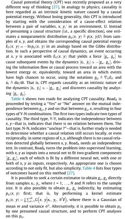
Experiments on the CauseEffectPairs (CEP) benchmark have demonstrated that a preliminary and simple implementation of CPT has achieved performances that are comparable with ones achieved by state-of-art methods.

Further development is to explore the estimation of causal structure between multiple variable distributions and multiple variables, possibly along two directions. One is simply integrating the methods in Table 4 into the famous Peter-Clark(PC)algorithm[28], especially on edges that are difficultly identified by independent and conditional independent tests. The other is turning the conditions that gyis uncorrelated (or independent) of x and that gxis uncorrelated (or independent) of y into multivariate polynomial equations,and adding the equations into the ρ-diagram equations in Ref. [26], e.g., Eq. (29) and Eq. (33), to get an augmented group of polynomial equations. Then, the well known Wen-Tsun Wu method may be adopted to check whether the equations have unique or a finite number of solutions.

5. Discovering causal information from observational data

Causality is a fundamental notion in science, and plays an important role in explanation, prediction, decision-making, and control [28,29]. There are two essential problems to address in modern causality research.One essential problem is the identification of causal effects, that is, identifying the effects of interventions, given the partially or completely known causal structure and some observed data; this is typically known as ‘‘causal inference.” For advances in this research direction,readers are referred to Ref. [29] and the references therein. In causal inference, causal structure is assumed to be given in advance—but how can we find causal structure if it is not given?A traditional way to discover causal relations resorts to interventions or randomized experiments,which are too expensive or time-consuming in many cases, or may even be impossible from a practical standpoint. Therefore,the other essential causality problem, which is how to reveal causal information by analyzing purely observational data,has drawn a great deal of attention [28].

In the last three decades,there has been a rapid spread of interest in principled methods causal discovery,which has been driven in part by technological developments. These technological developments include the ability to collect and store big data with huge numbers of variables and sample sizes, and increases in the speed of computers. In domains containing measurements such as satellite images of weather, functional magnetic resonance imaging(fMRI) for brain imaging, gene-expression data, or singlenucleotide polymorphism (SNP) data, the number of variables can range in the millions, and there is often very limited background knowledge to reduce the space of alternative causal hypotheses. Causal discovery techniques without the aid of an automated search then appear to be hopeless. At the same time, the availability of faster computers with larger memories and disc space allow for practical implementations of computationally intensive automated algorithms to handle large-scale problems.

It is well known in statistics that‘‘causation implies correlation,but correlation does not imply causation.”Perhaps it is fairer to say that correlation does not directly imply causation; in fact, it has become clear that under suitable sets of assumptions, the causal structure (often represented by a directed graph) underlying a set of random variables can be recovered from the variables’observed data,at least to some extent.Since the 1990s,conditionalindependence relationships in the data have been used for the purpose of estimating the underlying causal structure.Typical(conditional independence) constraint-based methods include the PC algorithm and fast causal inference (FCI) [28]. Under the assumption that there is no confounder (i.e., unobserved direct common cause of two measured variables),the result of PC is asymptotically correct. FCI gives asymptotically correct results even when there are confounders. These methods are widely applicable because they can handle various types of causal relations and data distributions, given reliable conditional independence testing methods.However,they may not provide all the desired causal information,because they output(independence)equivalence classes—that is,a set of causal structures with the same conditional independence relations. The PC and FCI algorithms output graphical representations of the equivalence classes. In cases without confounders,there also exist score-based algorithms that estimate causal structure by optimizing some properly defined score function. The greedy equivalence search (GES), among them, is a widely used two-phase procedure that directly searches over the space of equivalence classes.

Table 4 Two roads for analyzing CPT causality.

In the past 13 years, it has been further shown that algorithms based on properly constrained FCMs are able to distinguish between different causal structures in the same equivalence class,thanks to additional assumptions on the causal mechanism. An FCM represents the outcome or effect variable Y as a function of its direct causes X and some noise term E,that is,Y =f （X ，E）,where E is independent of X. It has been shown that, without constraints on function f, for any two variables, one of them can always be expressed as a function of the other and independent noise [30].However, if the functional classes are properly constrained, it is possible to identify the causal direction between X and Y because for wrong directions, the estimated noise and hypothetical cause cannot be independent (although they are independent for the right direction).Such FCMs include the LiNGAM[31],where causal relations are linear and noise terms are assumed to be non-Gaussian; the post-nonlinear (PNL) causal model [32], which considers nonlinear effects of causes and possible nonlinear sensor/measurement distortion in the data; and the nonlinear ANM[33,34], in which causes have nonlinear effects and noise is additive.For a review of these models and corresponding causal discovery methods, readers are referred to Ref. [30].

Causal discovery exploits observational data. The data are produced not only by the underlying causal process, but also by the sampling process. In practice, for reliable causal discovery, it is necessary to consider specific challenges posed in the causal and sampling processes, depending on the application domain. For example, for multivariate time series data such as mRNA expression series in genomics and blood-oxygenation-level-dependent(BOLD)time series in neuropsychology, finding the causal dynamics generating such data is challenging for many reasons,including nonlinear causal interactions, a much lower data-acquisition rate compared with the underlying rates of change, feedback loops in the causal model, the existence of measurement error, nonstationarity of the process, and possible unmeasured confounding causes. In clinical studies,there is often a large amount of missing data.Data collected on the Internet or in hospital often suffer from selection bias. Some datasets involve both mixed categorical and continuous variables, which may pose difficulties in conditional independence tests and in the specification of appropriate forms of the FCM. Many of these issues have recently been considered,and corresponding methods have been proposed to address them.

Causal discovery has benefited a great deal from advances in machine learning,which provide an essential tool to extract information from data.On the other hand,causal information describes properties of the process that render a set of constraints on the data distribution and is able to facilitate understanding and solve a number of learning problems involving distribution shift or concerning the relationship between different factors of the joint distribution. In particular, for learning under data heterogeneity, it is naturally helpful to learn and model the properties of data heterogeneity, which then benefit from causal modeling. Such learning problems include domain adaptation (or transfer learning) [35],semi-supervised learning, and learning with positive and unlabeled examples.Leveraging causal modeling for recommender systems and reinforcement learning is becoming an active research field in recent years.

6. Formal argumentation in causal reasoning and explanation

In this section, we sketch why and how formal argumentation can play an important role in causal reasoning and explanation.Reasoning in argumentation is realized by constructing, comparing, and evaluating arguments [36]. An argument commonly consists of a claim that may be supported by premises, which can be observations, assumptions, or intermediate conclusions of some other arguments. The claim, the premises, and the inference relation between them may be the subject of rebuttals or counterarguments [37]. An argument can be accepted only when it survives all attacks.In AI,formal argumentation is a general formalism for modeling defeasible reasoning. It provides a natural way for justifying and explaining causation, and is complementary to machine learning approaches,for learning,reasoning,and explaining cause-and-effect relations.

6.1. Nonmonotonicity and defeasibility

Causal reasoning is the process of identifying causality, that is,the relationship between a cause and its effect, which is often defeasible and nonmonotonic. On the one hand, causal rules are typically defeasible. A causal rule may be represented in the form‘‘c causes e” where e is some effect and c is a possible cause. The causal connective is not a material implication, but a defeasible conditional with strength or uncertainty. For example, ‘‘turning the ignition key causes the motor to start, but it does not imply it,since there are some other factors such as there being a battery,the battery not being dead,there being gas,and so on”[38].On the other hand, causal reasoning is nonmonotonic, in the sense that causal connections can be drawn tentatively and retracted in light of further information. It is usually the case that c causes e, but c and d jointly do not cause e. For example, an agent believes that turning the ignition key causes the motor to start, but when it knows that the battery is dead, it does not believe that turning the ignition key will cause the motor to start. In AI, this is the famous qualification problem. Since the potentially relevant factors are typically uncertain,it is not cost effective to reason explicitly. So, when doing causal inference, people usually ‘‘jump” to conclusions and retract some conclusions when needed. Similarly,reasoning from evidence to cause is nonmonotonic. If an agent observes some effect e,it is allowed to hypothesize a possible cause c.The reasoning from the evidence to a cause is abductive,since for some evidence, one may accept an abductive explanation if no better explanation is available. However, when new explanations are generated, the old explanation might be discarded.

6.2. Efficiency and explainability

From a perspective of computation, monotonicity is a crucial property of classical logic, which means that each conclusion obtained by local computation using a subset of knowledge is equal to the one made by global computation using all the knowledge.This property does not hold in nonmonotonic reasoning and,therefore, the computation could be highly inefficient. Due to the nonmonotonicity of causal reasoning, in order to improve efficiency,formal argumentation has been evidenced to be a good candidate,by comparing it with some other nonmonotonic formalisms such as default logic and circumscription.The reason is that in formal argumentation, computational approaches may take advantage of the divide-and-conquer strategy and maximal usage of existing computational results in terms of the reachability between nodes in an argumentation graph[39].Another important property of causal reasoning in AI is explainability. Traditional nonmonotonic formalisms are not ideal for explanation, since all the proofs are not represented in a human understandable way. Since the purpose of explanation is to let the audience understand, the cognitive process of comparing and contrasting arguments is significant [37]. Argumentation provides such a way by exchanging arguments in terms of justification and argument dialogue [40].

6.3. Connections to machine learning approaches

In explainable AI, there are two components: the explainable model and the explanation interface. The latter includes reflexive explanations that arise directly from the model and rational explanations that come from reasoning about the user’s beliefs.To realize this vision,it is natural to combine argumentation and machine learning, in the sense that knowledge is obtained by machine learning approaches,while the reasoning and explanation are realized by argumentation. Since argumentation provides a general approach for various kinds of reasoning in the context of disagreement,and can be combined with some uncertainty measures,such as probability and fuzziness,it is very flexible to model the knowledge learned from data.An example is when a machine learns features and produces an explanation, such as ‘‘This face is angry,because it is similar to these examples, and dissimilar from those examples.”This is an argument,which might be attacked by other arguments. And, in order to measure the uncertainty described by some words such as‘‘angry,”one may choose to use possibilistic or probabilistic argumentation[41].Different explanations may be in conflict. For instance, there could be some cases invoking specific examples or stories that support a choice, and rejections of an alternative choice that argue against less-preferred answers based on analytics,cases,and data.By using argumentation graphs,these kinds of support-and-attack relations can be conveniently modeled and can be used to compute the status of conflicting arguments for different choices.

7. Causal inference with complex experiments

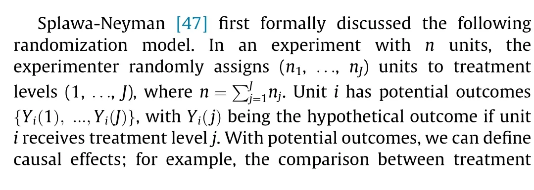
The potential outcomes framework for causal inference starts with a hypothetical experiment in which the experimenter can assign every unit to several treatment levels.Every unit has potential outcomes corresponding to these treatment levels. Causal effects are comparisons of the potential outcomes among the same set of units. This is sometimes called the experimentalist’s approach to causal inference [42]. Readers are referred to Refs.[43-46], for textbook discussions.

7.1. Randomized factorial experiments

7.2. The role of covariates in the analysis of experiments

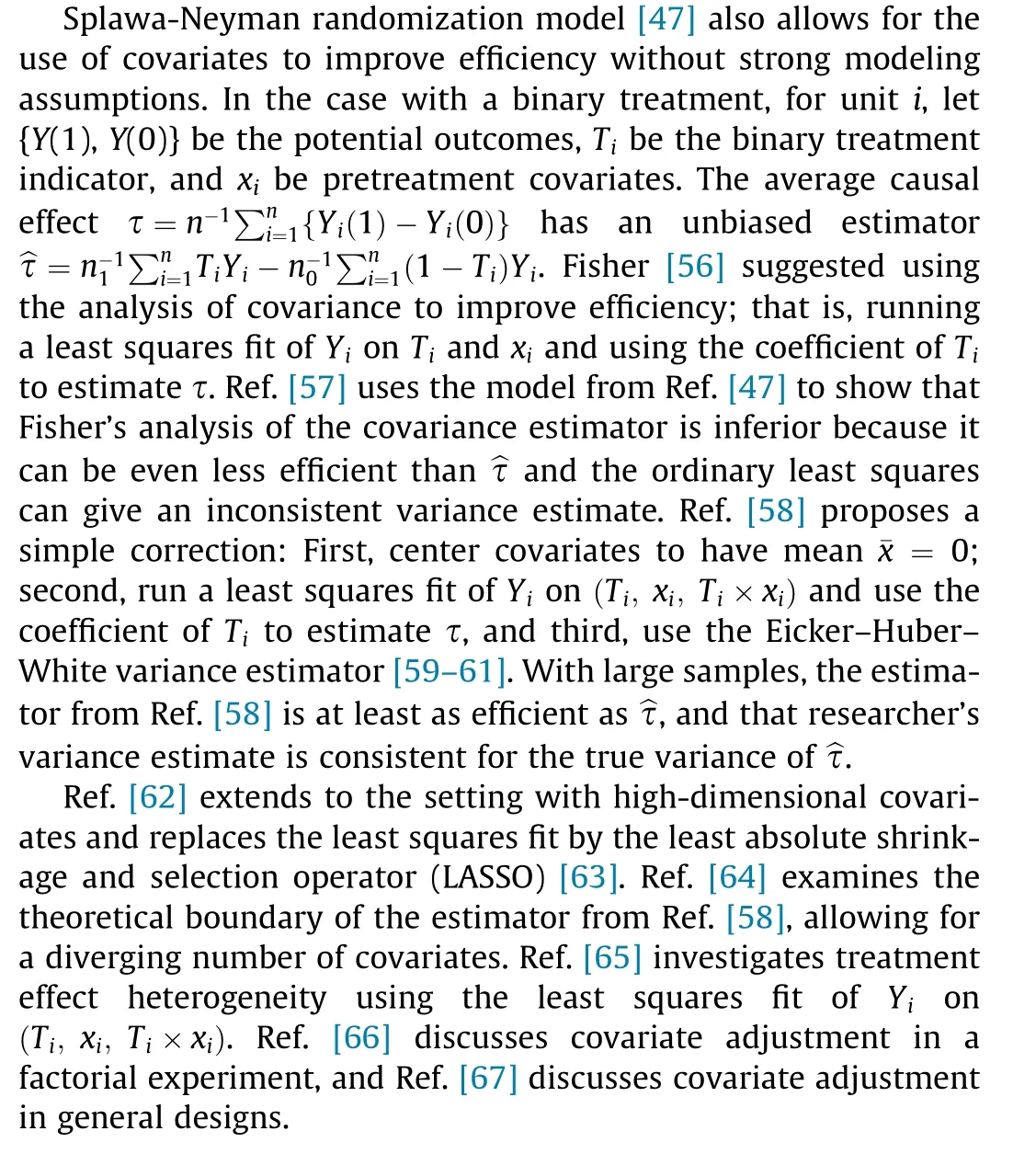
7.3. The role of covariates in the design of experiments

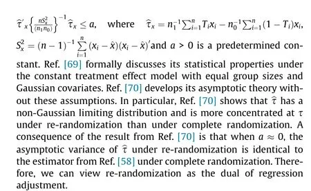
Ref. [71] proposes a re-randomization scheme that allows for tiers of covariates, and Ref. [70] derives its asymptotic properties.Refs. [72,73] extend re-randomization to factorial experiments,and Ref. [74] proposes sequential re-randomization.

7.4. Final remarks

Following Ref. [47], I have focused on the repeated sampling properties of estimators with randomized experiments. Alternatively, Fisher randomization tests are finite-sample exact for any test statistics and for any designs,under the sharp null hypothesis that Yi（1 ）=···=Yi（J ） for all units i = 1, ..., J [46,75,76]. Refs.[77,78] propose the use of covariate adjustment in randomization tests,and Ref.[69]proposes the use of randomization tests to analyze re-randomization. Refs. [79-81] apply randomization tests to experiments with interference.Refs.[48,50,82]discuss the properties of randomization tests for weak null hypotheses.Refs.[83-85]invert randomization tests to construct exact confidence intervals.Finally, Ref. [86] discusses different inferential frameworks from the missing data perspective.

8. Instrumental variables and negative controls for observational studies

In a great deal of scientific research, the ultimate goal is to evaluate the causal effect of a given treatment or exposure on a given outcome or response variable. Since the work published in Ref. [75], randomized experiments have become a powerful and influential tool for the evaluation of causal effects; however, they are not feasible in many situations due to ethical issues,expensive cost, or imperfect compliance. In contrast, observational studies offer an important source of data for scientific research. However,causal inference with observational studies is challenging,because confounding may arise.Confounders are covariates that affect both the primary exposure and the outcome.In the presence of unmeasured confounders,statistical association does not imply causation,and vice versa, which is known as the Yule-Simpson paradox[19,20].Refs.[87,88]review the concepts of confounding,and Refs.[2,89,90] discuss methods for the adjustment of observed confounders,such as regressing analysis,propensity score,and inverse probability weighting,as well as doubly robust methods.Here,we review two methods for the adjustment of unmeasured confounding: the instrumental variable approach and the negative control approach.

Throughout,we let X and Y denote the exposure and outcome of interest, respectively, and we let U†† In this section, we reuse U to denote the unmeasured confounders. Please note that, U was used to denote an environment in Section 4.denote an unmeasured confounder; for simplicity, we omit observed confounders, which can be incorporated in the following by simply conditioning on them.We use lowercase letters to denote realized values of random variables—for example, y for a realized value of Y.

The instrumental variable approach, which was first proposed in econometrics literature in the 1920s [91,92], has become a popular method in observational studies to mitigate the problem of unobserved confounding. In addition to the primary treatment and outcome, this approach involves an instrumental variable Z that satisfies three core assumptions:

(1) It has no direct effect on the outcome, that is, Z ⊥Y| （X ， U）(exclusion restriction);

(2) It is independent of the unobserved confounder, that is,Z ⊥U (independence);

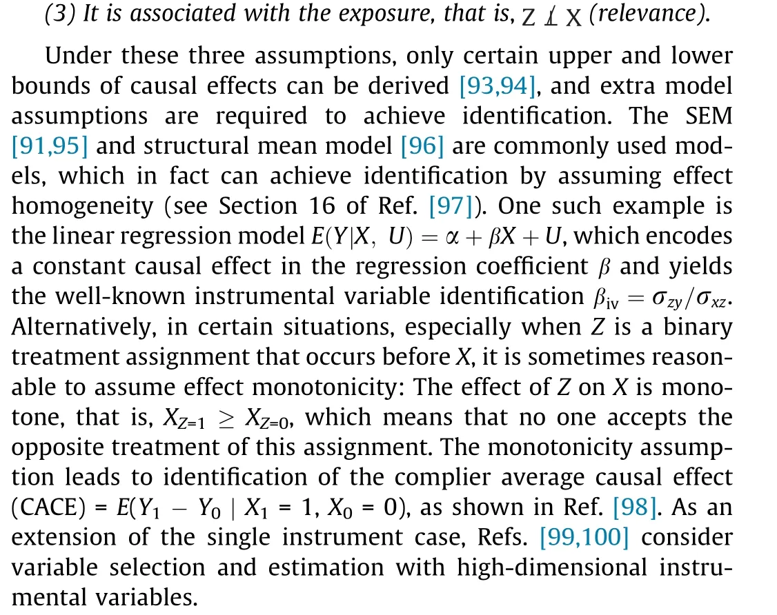
However, in practice, the instrumental variable assumptions may not be met, and the approach is highly sensitive to the violation of any of them. Validity checking and violation detection of these assumptions are important before applying the instrumental variable approach, and have been attracting researchers’ attention[94,101]. In case of a violation of the core assumptions, identification of the causal effect is often impossible,and bounding and sensitivity analysis methods [102,103] have been proposed for causal inference.

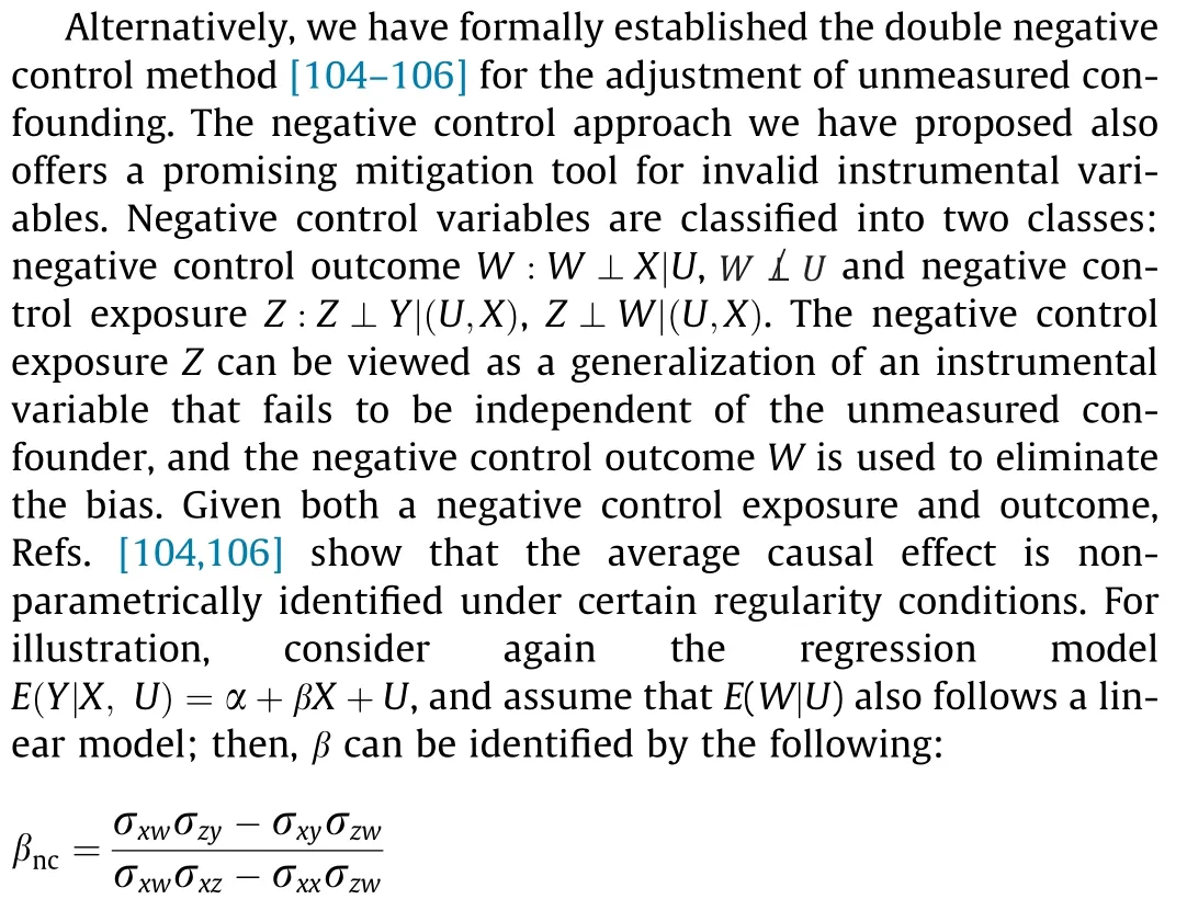
This formula does apply to a valid instrumental variable; in which case,Z ⊥U,and thus,σzw=0,according to the negative control outcome assumption. Therefore, the instrumental variable identification can be viewed as a special case of the negative control approach. However, in contrast to the instrumental variable,negative controls require weak assumptions that are more likely to hold in practice. Refs. [107,108] provide elegant surveys on the existence of negative controls in observational studies. Refs.[105,109] point out that negative controls are widely available in time series studies, as long as no feedback effect is present, such as studies about air pollution and public health.

Refs. [107,109,110] examine the use of negative controls for confounding detection or bias reduction when a solely negative control exposure or outcome is available but are unable to achieve identification.Refs.[111,112]propose the use of multiple negative control outcomes to remove confounding in statistical genetics but must rest on a factor analysis model.

9. Causal inference with interference

The stable unit treatment value assumption plays an important role in the classical potential outcomes framework.It assumes that there is no interference between units[76].However,interference is likely to be present in many experimental and observational studies,where units socially or physically interact with each other.For example,in educational or social sciences,people enrolled in a tutoring or training program may have an effect on those not enrolled due to the transmission of knowledge [113,114]. In epidemiology, the prevention measures for infectious diseases may benefit unprotected people by reducing the probability of contagion [115,116]. In these studies, one unit’s treatment can have a direct effect on its own outcome as well as a spillover effect on the outcome of other units. The direct and spillover effects are of scientific or societal interest in real problems; they enable an understanding of the mechanism of a treatment effect,and provide guidance for policy making and implementation.

In the presence of interference, the number of potential outcomes of a unit grows exponentially with the number of units.†† If the total number of units is N, then there are 2N potential outcomes for each unit.As a result,it is intractable to estimate the direct and spillover effects without restriction in the literature on the estimation of treatment effects with interference structure.There has been a rapidly growing interest in interference (see Ref. [117] for a recent review). A significant direction of work focuses on limited interference within nonoverlapping clusters and assumes that there is no interference between clusters [52,114,118-122]. This is referred to as the partial interference assumption [114]. Recently, several researchers have considered the relaxation of the partial interference assumption to account for a more general structure of interference (e.g., Refs.[123-126]). The variance estimation is more complicated under interference. As pointed out in Ref. [118], it is difficult to calculate the variances for the direct and spillover effects even under partial interference.In model-free settings,a typical assumption for obtaining valid variance estimation is that the outcome of a unit depends on the treatments of other units only through a function of the treatments. Ref. [118] provides a variance estimator under the stratified interference assumption, and Ref. [124] generalizes it under a weaker assumption.

Another direction of work targets new designs to estimate treatment effects based on the interference structure. Under the partial interference assumption, Ref. [118] proposes the twostage randomized experiment as a general experimental solution to the estimation of the direct and spillover effects. In more complex structures such as social networks,researchers have proposed several designs for the point and variance estimation of the treatment effects [127-129].

For the inference under interference, Refs. [130,131] rely on models for the potential outcomes.Ref.[79]develops a conditional randomization test for the null hypothesis of no spillover effect.Ref.[80]extends this test to a larger class of hypotheses restricted to a subset of units, known as focal units. Building on this work,Ref. [132] provides a general procedure for obtaining powerful conditional tests.

Interference brings up new challenges. First, the asymptotic properties require advanced techniques deriving. Ref. [133] investigates the consistency of the difference in the means estimator when the number of the units that can be interfered with does not grow as quickly as the sample size.Ref.[134]develops the central limit theorem for direct and spillover effects under partial interference and stratified interference.Ref.[52]provides the central limit theorem for a peer effect under partial interference and stratified interference. However, under general interference, the asymptotic properties remain unsolved—even for the simplest difference in the means estimator.Second,interference becomes even harder to deal with when data complications are present. Refs.[120,121,135,136] consider noncompliance in an interference setting. Ref. [137] examines the censoring of time-to-event data in the presence of interference. However, for other data complications such as missing data and measurement error, no methods are yet available.Third,most of the literature focuses on the direct effect and the spillover effect. However, interference may be present in other settings, such as mediation analysis (see Ref. [138]for a mediation analysis under interference)and longitudinal studies,where different quantities are of interest. As a result,it is necessary to generalize the commonly used methods in these settings to account for the interference between units.

Compliance with ethics guidelines

Kun Kuang, Lian Li, Zhi Geng, Lei Xu, Kun Zhang, Beishui Liao,Huaxin Huang, Peng Ding, Wang Miao, and Zhichao Jiang declare that they have no conflict of interest or financial conflicts to disclose.