Study on the Predication Modeling of COD for Water Based on UV-VIS Spectroscopy and CNN Algorithm of Deep Learning

JIA Wen-shen, ZHANG Heng-zhi, MA Jie, LIANG Gang, WANG Ji-hua, LIU Xin

1. Beijing Research Center of Agricultural Standards and Testing， Beijing 100097， China 2. Beijing Information Science and Technology University， Beijing 100192， China 3. Technical Center， Beijing Customs District, Beijing 100026， China 4. Department of Risk Assessment Lab for Agro-products， Beijing 100097， China 5. Key Laboratory of Urban Agriculture (North China), Ministry of Agriculture and Rural Affairs, Beijing 100097, China

Abstract Water is vital for human life, and the quality of water is directly related to people’s quality of life. At present, research into chemical oxygen demand (COD) methods for determining water quality is mainly focused on spectral data preprocessing and spectral feature extraction, with few studies considering spectral data modeling methods. Convolutional neural networks (CNN) are known to have strong feature extraction and feature mapping abilities. Thus, in this study, a CNN is combined with UV-visible spectroscopy to establish a COD prediction model. The Savitzky-Golay smoothing filter is applied to remove noise interference, and the spectral data are then input to the CNN model. The features of the spectrum data are extracted through the convolution layer, the spatial dimensions are reduced in the pooling layer, and the global features are mapped in the fully connected layer. The model is trained using the ReLU activation function and the Adam optimizer. A series of experiments show that the CNN model has a strong ability to predict COD in water, with a high prediction accuracy and good fit to the regression curve. A comparison with other models indicates that the proposed CNN model gives the smallest RMSEP and MAE, the largest -R2, and the best fitting effect. It is found that the model has strong generalization ability through the evaluation effect of the training samples. To counter the inaccuracy of the predicted results caused by the peak shift of the absorption spectrum, a regression model based on a strengthened CNN (CNNs) is also developed. After denoising, the spectral data can be divided into three categories according to the different characteristics of absorption peaks, and the corresponding CNN regression model is input respectively for prediction. When the corresponding regression model is applied, the experimental results show that the sectional CNNs model outperforms our original CNN model in terms of fitting, prediction precision, determination coefficient, and error. Not only does R2 increase significantly, reaching 0.999 1, but also the MAE and RMSEP of the test samples also reduced to 2.314 3 and 3.874 5, respectively, which were reduced by 25.9% and 21.33% compared with out original CNN. Performance testing of the prediction model, indicates that the detection limit is 0.28 mg·L-1and the measurement range is 2.8～500 mg·L-1. This paper describes an innovative combination of a CNN with spectral analysis and reports our pioneering ideas on the application of spectral analysis in the field of water quality detection.

Keywords Ultraviolet visible spectrum; Convolution neural network; Chemical oxygen demand; Prediction model

Introduction

Over recent decades, the acceleration of urbanization has led to a dramatic rise in water pollution issues[1]. Therefore, the real-time remote detection of the degree of water pollution, rapid and accurate detection of pollution areas, and timely and effective prevention of water pollution have become key components in the control of water pollution. The chemical oxygen demand (COD) is an important indicator for assessing the degree of pollution of water bodies[2-3]and is widely used in the detection of water pollution. COD refers to the mass concentration of oxygen in strong oxidants (such as potassium dichromate, potassium permanganate) consumed by dissolved substances and suspended matter in the water. High content of COD indicates, the higher the concentration of reducing substances in the water, and the more severe the level of pollution[4-5].

At present, studies on water quality COD detection methods are mainly focused on spectral data preprocessing and spectral feature extraction[6-8], with relatively little research on spectral data modeling methods by deep learning. Deep learning has gradually gained popularity in various fields, exhibiting strong performance in commercial applications such as speech recognition, image recognition, and recommendation systems[9], and performing very well in food safety, drug discovery, and genomics[10-11].

As a common deep learning model type, convolutional neural networks (CNN) extract high-dimensional data features through multi-level convolution operations and reduce the dimensionality to produce low-dimensional features through the pooling layer. They perform well in feature mapping[12]. In this study, a CNN is combined with UV-visible spectroscopy to give a CNN-based detection method for water COD UV-visible spectroscopy. The proposed model first removes spectral noise using a Savitzky-Golay smoothing filter[13-14], and then inputs the denoised spectral data into the CNN model for feature extraction and COD prediction. Compared with backpropagation (BP)[15-16], principal component analysis BP (PCA-BP)[17], partial least-squares regression (PLSR)[18-19], and random forest (RF)[20]models, CNN can achieve higher prediction ability. On this basis, a strengthened CNN-based classification regression model (CNNs) is proposed. This divides the denoised spectral data into three categories through the CNN classification model, and inputs the corresponding CNN regression model for prediction. Experimental results show that the segmented CNNs model produces better performance and higher prediction accuracy than the global CNN model. This method is of great significance for the application of deep learning in water COD detection.

1 Description of Algorithms

1.1 Savitzky-Golay Smoothing Filters

During the modeling, the large amount of noise contained in the spectral data signal was found to interfere with the extracted features[21]. Experiments showed that Savitzky-Golay smoothing filters could effectively remove noise interference. This preprocessing method, which is commonly used in spectral analysis, is based on polynomial least-squares fitting and ensures the integrity of the original data while filtering out the noise, effectively providing data support for modeling.

1.2 Principles of CNN

CNN differ from general neural networks, having a deeper network structure and featuring local connections and weight sharing. These modifications greatly reduce network complexity and provide a more powerful feature mapping capability[22-23]. As shown in Figure 1, CNN consist of a convolutional layer, a pooling layer, and a fully connected layer.

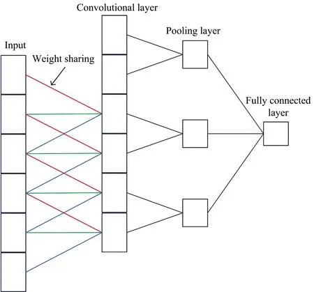
Fig.1 Fundamental structure of CNN

The convolutional layer convolves the feature map of the previous layer through the convolution kernel:

(1)

wherekis the convolution kernel,lis the number of layers,Mjis thejthfeature map, and b is the offset. By performing convolution to extract different characteristics of the input data, the input data can be reduced from high- to low-dimensional feature space, thus reducing the dimensionality of the data. To improve the characterization performance of the network, an activation layer is added between the convolutional layer and the pooling layer to convert the output of the upper layer into a finite value through a nonlinear activation function, giving the gradient-based optimization method faster convergence and greater stability. Commonly used activation functions include the sigmoid, tanh, and ReLU functions. The role of the pooling layer is to down-sample the output data from the previous layer, while retaining useful feature information. This not only reduces the data size, but also improves the generalization ability of the network. The fully connected layer is equivalent to a multilayer perceptron[24]. Each of its neurons is connected to the neurons of the previous layer, and all of the extracted features are combined. The convolutional layer, pooling layer, and activation layer map the input raw data to the hidden layer feature space, while the fully connected layer maps the learned distributed feature representation to the sample labels.

2 Experiment

2.1 Data Collection and Processing

Water samples were obtained from potassium hydrogen phthalate standard samples of different concentrations prepared by the National Nonferrous Metals and Electron Materials Analysis and Testing Center. Some of the water samples were diluted with pure water. Finally, a total of 200 water samples were obtained, and the true COD values of the water samples ranged from 0～500 mg·L-1. The UV-visible absorption spectra collected from these samples are shown in Figure 2.

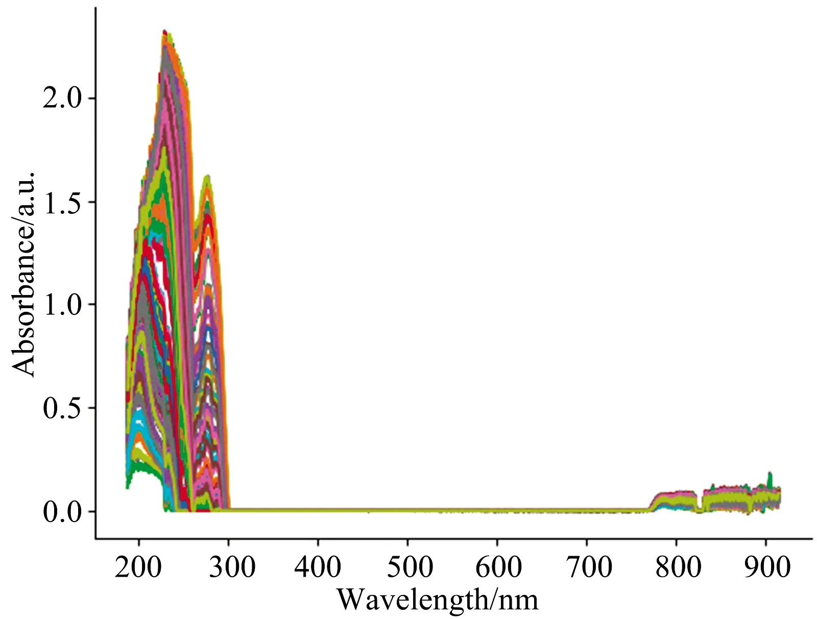
Fig.2 Collected UV-Visible absorption spectra

The absorbance was measured using a BIM-6002A Spectroscopic Detector (Brolight, China). This detector adopts a cross-symmetric C-T optical path structure with an optical resolution of 0.35～1 nm, a minimum integration time of 0.5 ms, and an operating wavelength range of 188～915 nm, and has a total of 2 048 detection sites. It takes an average of 10 measurements and subtracts the dark spectrum[25]. That is, no spectral data are output by the spectrum detector when there is no water sample or no light source, thus ensuring the accuracy of the data. The resulting spectral data were filtered using Savitzky-Golay smoothing filters to reduce noise interference.

2.2 Building the Prediction Model

The Keras deep learning framework was used to build a CNN-based water quality COD prediction model, with all programming performed in Python[26]. The CNN model structure is shown in Figure 3. It consists mainly of a convolutional layer, pooling layer, and fully connected layer. First, the denoised spectral data were converted into a 2 048×1 spectral matrix. The first convolutional layer had two 9×1 convolution kernels to extract spectral features. The obtained feature maps[27]were then subsampled after the activation layer. The pooling layer had a window size of 2. Average pooling was conducted to reduce the number of parameters while guaranteeing no loss of feature information. The pooling process generated half of the spectral data. The dimensionality of the spectral data was reduced while the spectral features were extracted.

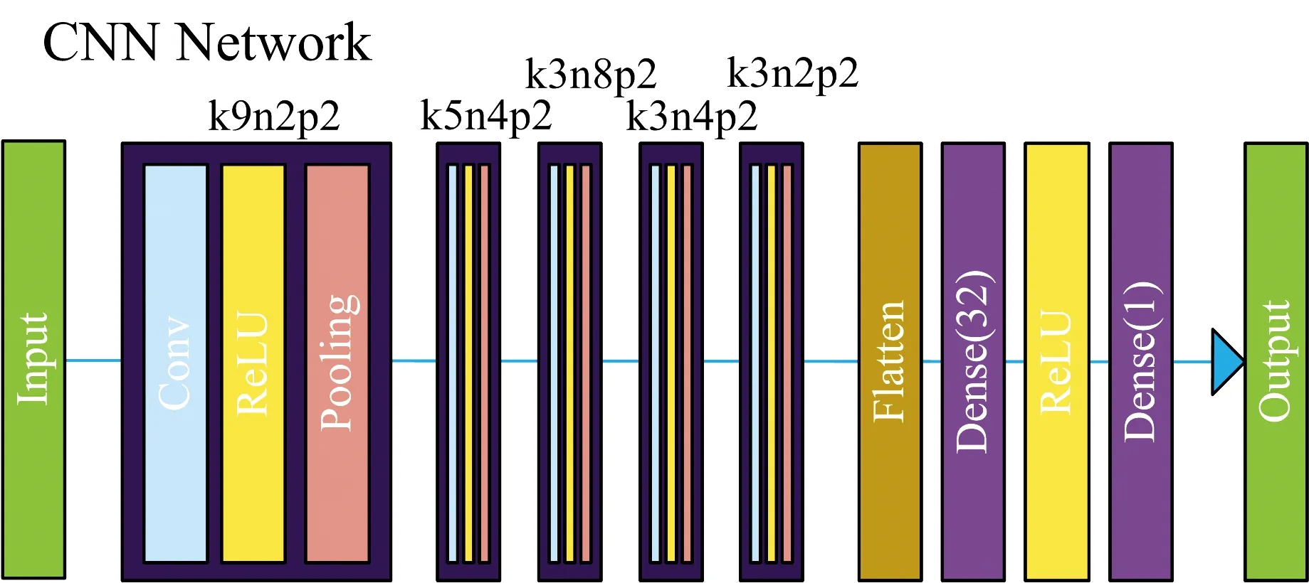
Fig.3 CNN network structure and kernel size (k) corresponding to each convolutional layer, the number of feature maps (n), and the window size of the pooling layer (p)

The ReLU activation function was employed in the activation layer[28]. ReLU changes all input negative numbers to 0, and does not change the value of non-negative numbers. This one-sided suppression makes the function output sparse, preventing over-fitting due to excessive parameters[29]. As the gradient of the non-negative interval is constant and non-zero, the convergence is relatively stable.

To identify the significant spectral characteristics, after the first convolutional layer and the pooling layer, convolutions were sequentially performed through convolutional layers with kernel sizes of 5×1, 3×1, 3×1, 3×1, and pooling was conducted through the pooling layer with a window width of 2. The continuous convolution and pooling process not only smooths the high-frequency noise of the spectrum, but also reduces the dimensionality of the data while retaining the feature information. In addition, because the CNN has the characteristics of weight sharing and local perception, the network has relatively few parameters. Before entering the fully connected layer, the multidimensional data were flattened through the flattening layer. Regression fitting of the spectral feature vectors was conducted by passing the resulting one-dimensional data through the fully connected layer. The final output was the predicted COD value.

2.3 Model Training

All samples were divided into training sets and test sets according to a 9∶1 ratio. The training sets were used to train the model and update the weights. During each training process, 10% of the samples were randomly selected as verification set to monitor the training effect of the model and facilitate the optimization. The test sets were used to evaluate the training results of the model. Each sample corresponded to a true COD value. To prevent model overfitting, the test set was not used in the training stage.

After repeated experiments, the training learning rate was set to 0.01, the number of batches was set to 16, and the number of iterations was set to 300. Network weights and offsets were randomly initialized. The mean absolute error (MAE) was used as the loss function of the model. MAE is a commonly used regression loss function that measures the average error in the predicted values. Assuming that the input data isx, the CNN model determines a feature mapping functionf(x) to the water COD value. The purpose of the training was to find the optimal thresholdθthat minimizes the average absolute error off(x) (the predicted COD value) from the expected valuey(the true COD value):

(2)

To minimizeJ(θ) and find the optimal solution of the function, adaptive moment estimation (Adam)[30]was used as the training algorithm. The process of updating the Adam parameters is not affected by the expansion and contraction of the gradient, making this technique suitable for solving problems with high-noise, sparse-gradient spectral data. Thus, the training process only requires fine-tuning.

During the training stage, the loss function of the verification set was monitored. If the loss function did not decrease over 15 consecutive epochs, the training learning rate was reduced to 1/10, which solved the problem of the loss function oscillating without converging.

3 Results and Discussion

3.1 Prediction Model Evaluation

The 200 samples were divided into sets of 180 training samples and 20 test samples, with the training samples and the test samples having the same distribution. Then, BP, PCA-BP, PLSR, RF, and CNN models were trained and tested using the same training sets and test sets. The decision coefficientR2was used to evaluate the goodness of fit of each model. The root mean square error of calibration (RMSEC), root-mean-square error of prediction (RMSEP)[31], MAE, and mean absolute percentage error MAPE[32-33]were used as indicators of the models’ accuracy. Larger values ofR2and smaller values of RMSEP, MAE, and MAPE indicate better prediction by a model. After the training and testing had been repeated 10 times, the average results were obtained. These results are presented in Table 1.

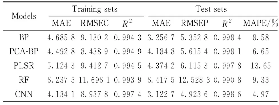
Table 1 Evaluation of the Prediction effect of the models

In terms of the model goodness of fit using the test samples, CNN has the largestR2(reaching 0.998 6), followed by BP (0.998 4). RF has the worst fitting effect,R2only 0.990 8. In terms of the accuracy of the model on the test samples, CNN produced the smallest RMSEP and MAE values, indicating that the predicted value is closer to the observed value than in the other models. To measure the ratio between the error and the true value, MAPE was used as a key indicator for evaluating the models’ accuracy. A smaller MAPE value indicates that the model has higher prediction accuracy. The MAPE of CNN is 4.97%, which is the smallest value achieved by any of the models, indicating the highest precision. The effect evaluation of the test samples measures the predictive power of the models, whereas the evaluation of the effect of the training samples evaluates the generalization ability of the models[34]. By comparing the training effects of the training samples and the test samples, it was found that the effect evaluation on the test samples of the five models was better than the evaluation of the training samples, indicating that the models have strong generalization ability and no problems with overfitting.

In addition, the CNN model has certain data preprocessing capabilities. With other linear models and common nonlinear models, it is generally necessary to preprocess and denoise the spectral data before they are input into the model to reduce the noise interference. However, while removing the spectral noise, some spectral features will inevitably be lost, which will negatively affect the prediction accuracy of the model. Research shows that CNN offer excellent prediction accuracy, even without spectral preprocessing, as a result of their strong feature extraction capability and sample mapping of local features[35]. As shown in Figure 4, the RMSEP values of the test samples decreased for all models after denoising (Savitzky-Golay smoothing filter). Compared with the other models, the CNN model has the smallest difference before and after denoising and the lowest dependence on spectral data preprocessing. Thus, the CNN not only simplifies the prediction process, but also reduces noise interference and ensures high prediction accuracy.

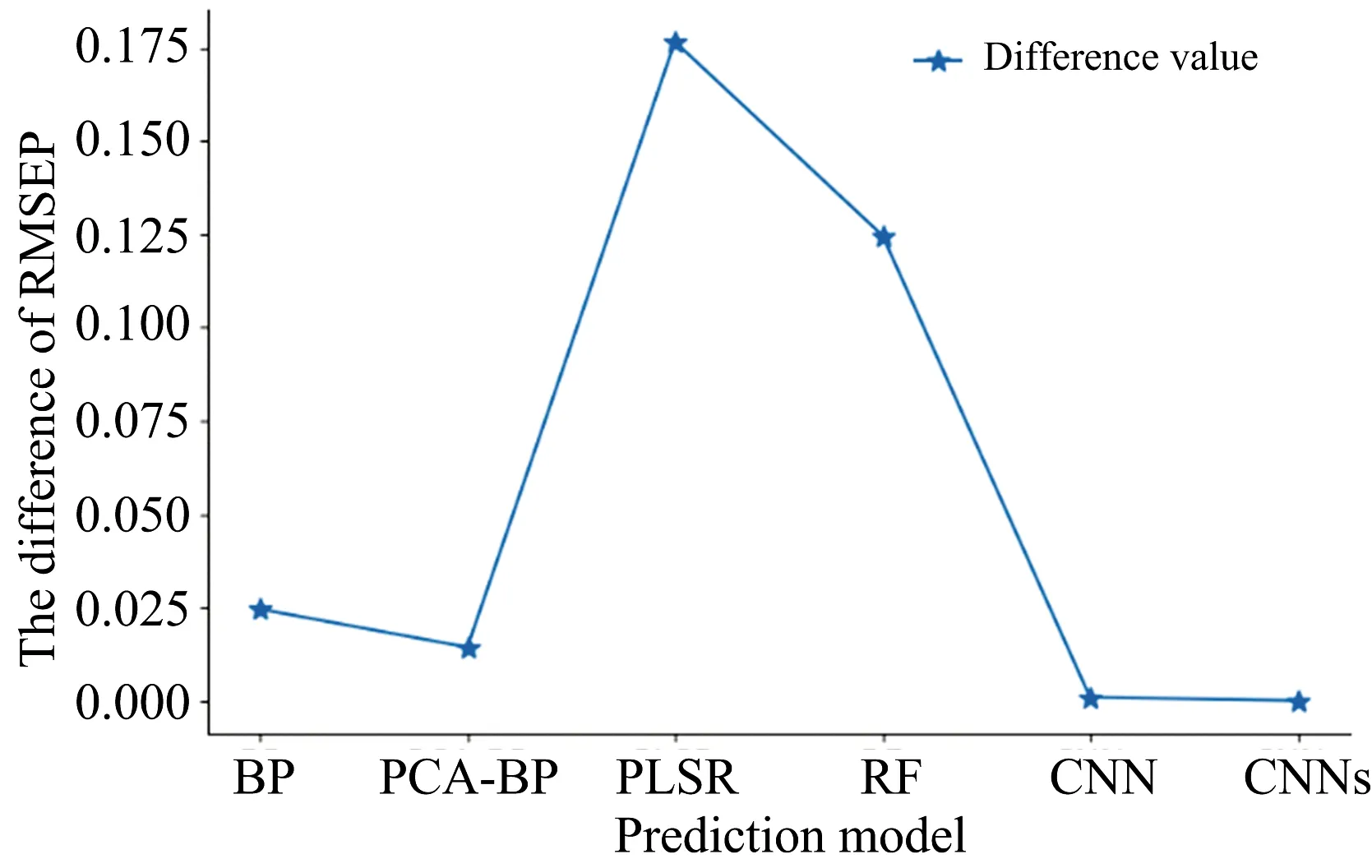
Fig.4 The difference between RMSEP before and after denoising of each prediction model

Through the above analysis, it was concluded that CNN provides accurate water COD predictions with good fit to the regression line. In predicting COD in new samples, the proposed CNN has good generalization ability and, compared with BP, PCA-BP, PLSR, and RF, is a highly efficient prediction model. However, although CNN works better than these other models, it still needs to be improved. In terms of model complexity and model parameters, our CNN has 4 263 weighting parameters, which is somewhat less than the 65 601 of BP but far higher than the 78 of PCA-BP. The prediction effect of these additional parameters is not significant. Therefore, an optimized CNN was developed.

3.2 Model Optimization

Compared with other neural networks, CNN have a deep network structure, more local connections, and better weight sharing. Although the network is complex, it has a strong feature mapping capability. Studies have shown that, under certain circumstances, a deeper CNN model structure strengthens the feature mapping ability of the model. However, an increase in the number of model network layers increases the risk of overfitting, and therefore requires a large number of training samples[36]. In practical applications, the experimental conditions and environmental factors mean that there is no guarantee of obtaining sufficient samples. Developing a high-performance predictive model is often problematic in practice when there are few samples or the sample sets are imbalanced.

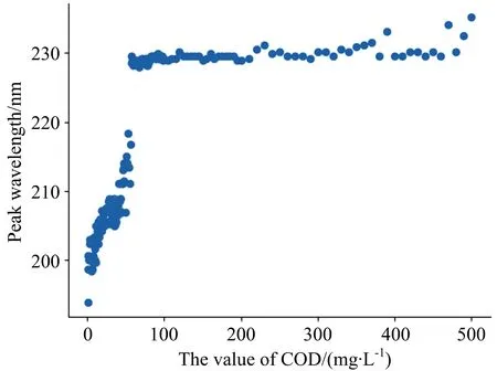
Fig.5 Relationship between COD value and peak wavelength

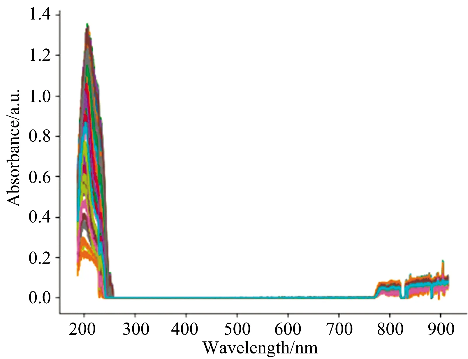
Fig.6 UV-Visible absorption spectra

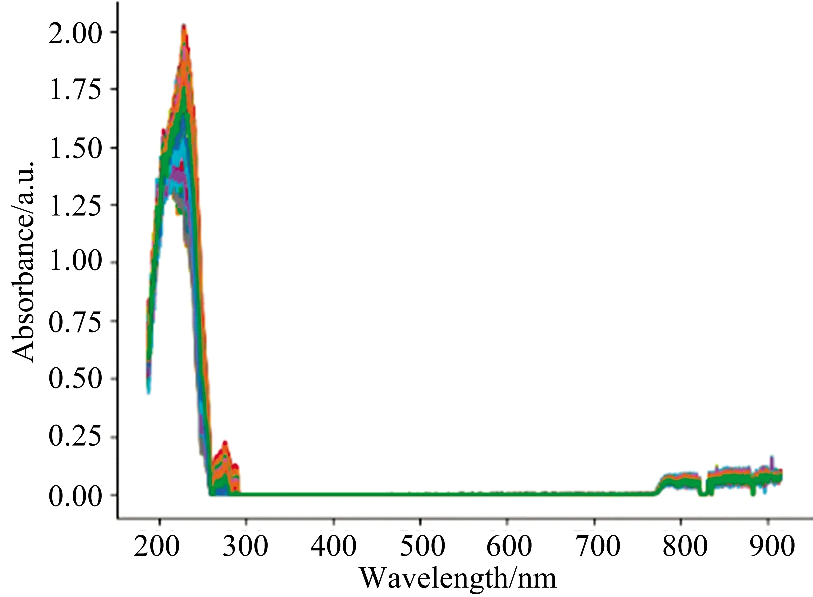
Fig.7 UV-Visible absorption spectra

As shown in Figure 5, the peak wavelength of the true COD values within the range 0～56 mg·L-1increases sharply as the COD content increases, whereas the peak wavelength of the COD content changes very little within the range 56～500 mg·L-1. As can be seen from Figure 2, with an increase in COD content, the crest shifts to the right, but the migration process is irregular and abrupt changes appear around the crest. The prediction model was divided into 0～56 mg·L-1and 56～500 mg·L-1for training and prediction according to the relationship between the peak wavelength and COD content. This experiment has shown that the model finds it difficult to converge during the training process because of irregular peak migration.

Fig.8 UV-Visible absorption spectra

To overcome the above problems, this paper proposes a segmentation prediction model called the strengthened CNN

(CNNs). This is a CNN-based classification regression model. First, the denoised spectral data are divided into three categories through the CNN classification model, and each category of data is then input into the corresponding CNN regression model for prediction. Model Ⅰ predicts COD at 0～45 mg·L-1, model Ⅱ predicts COD at 45～100 mg·L-1, and model Ⅲ predicts COD at 100～500 mg·L-1. The network structure of CNNs is shown in Figure 9.

The network structure of CNNs consists of two parts, a classification model and a regression model. The fully connected layer in the classification model uses the Softmax activation function[36]. Its output is the relative probability between different categories. The samples are classified according to the probability size and are assigned to the regression models with high probability. The classification model is tested after training, and the accuracy of the classification model reaches 100%, indicating that the classification model can accurately classify the input spectral data. The classified spectral data are input into the corresponding regression model according to the classification, and the training of the regression model is performed according to the true value of the sample.

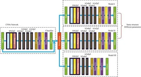
Fig.9 CNNs network structure and kernel size (k) corresponding to each convolution layer,number of feature maps (n), and window width of pooling layer (p)

Table 2 Evaluation of model prediction performance

Table 2 indicates that CNNs achieves outstanding performance compared to BP, PCA-BP, PLSR, and RF using the same training samples and test samples. Not only doesR2increase significantly, reaching 0.999 1, but the MAE and RMSEP of the test samples also decrease by 0.808 4 and 1.049 1, respectively, compared with our original CNN, and this effect is significant. The segmentation modeling and ability of the regression model to make parallel predictions mean that the number of model parameters is twice that in our original CNN. By comparing the model effect evaluation of test samples and training samples, the enhanced CNNs not only offers better prediction capabilities, but also achieves improved accuracy and stronger generalization ability.

3.3 Performance Test

To further verify the performance of the CNN prediction model, the detection limit and measurement range were tested. The COD content of a blank solution (pure water) was continuously measured seven times, and the standard deviation was calculated to be 0.094 163. The detection limit is three times the standard deviation, i.e., 0.28 mg·L-1. The lower limit of the COD value is 10 times the detection limit, so the lower limit of the measurement range is 2.8 mg·L-1. As the maximum concentration of the training samples in the model is 500 mg·L-1, the upper limit of the measurement range is 500 mg·L-1. Thus, the measurement range is 2.8～500 mg·L-1.

4 Conclusion

For the detection of water COD through UV-visible spectroscopy, a CNN model was used to establish a character mapping function between the water COD UV-visible spectrum and water COD content. After removing noise in the samples through Savitzky-Golay smoothing filters, the denoised spectral data were input into the CNN model for feature extraction and COD prediction. Experimental results show that the prediction power of our CNN is higher than that of other modeling methods. On this basis, a classification regression model was developed in which the spectral data are divided into three categories according to the COD concentration and input into the corresponding CNN regression model for prediction. The experimental results show that the segmented CNNs model achieves better performance and higher prediction accuracy than the global CNN model. This method combines CNNs with spectral analysis to provide an exploratory study for the application of deep learning methods in water quality testing.