Nonlinear amplitude versus angle inversion for transversely isotropic media with vertical symmetry axis using new weak anisotropy approximation equations

Lin Zhou · Zhuo‑Chao Chen · Jing‑Ye Li · Xiao‑Hong Chen · Xing‑Ye Liu · Jian‑Ping Liao

Abstract In VTI media, the conventional inversion methods based on the existing approximation formulas are difficult to accurately estimate the anisotropic parameters of reservoirs, even more so for unconventional reservoirs with strong seismic anisotropy.Theoretically, the above problems can be solved by utilizing the exact re flection coefficients equations. However, their complicated expression increases the difficulty in calculating the Jacobian matrix when applying them to the Bayesian deterministic inversion. Therefore, the new reduced approximation equations starting from the exact equations are derived here by linearizing the slowness expressions. The relatively simple form and satisfactory calculation accuracy make the reduced equations easy to apply for inversion while ensuring the accuracy of the inversion results. In addition, the blockiness constraint, which follows the differentiable Laplace distribution, is added to the prior model to improve contrasts between layers. Then, the concept of GLI and an iterative reweighted least-squares algorithm is combined to solve the objective function. Lastly, we obtain the iterative solution expression of the elastic parameters and anisotropy parameters and achieve nonlinear AVA inversion based on the reduced equations. The test results of synthetic data and field data show that the proposed method can accurately obtain the VTI parameters from prestack AVA seismic data.

Keywords Transversely isotropic media with vertical symmetry axis (VTI) · New reduced approximation equations ·Differentiable Laplace distribution · Blockiness constraint

1 Introduction

Amplitude variation with offset (AVO) or amplitude variation with incidence angle (AVA) inversion can provide more reliable elastic information of the subsurface for us. Therefore, the AVO/AVA inversion methods have been widely applied in the field of data inversion (Rutherford and Williams 1989; Ikelle 1995). Shale gas is one area where AVO/AVA inversion can greatly aid in the development of this unconventional hydrocarbon resource because of the diffi-culty in correctly depicting the subsurface. In the absence of fractures, many shales can be approximated as transversely isotropic with a vertical axis of symmetry (VTI), and their anisotropy feature is usually relatively strong (Rüger 1996;Sayers 2005; Bachrach 2015; Wang 2002; Zhang and Li 2013, 2016), which significantly affects the applicability and accuracy of the conventional AVA inversion. The re flection coefficient equation is the basis of AVA inversion,and its calculation accuracy will directly affect the accuracy of inversion results. Henneke (1972), Keith and Crampin(1977), Daley and Hron (1977) and Rüger (1996) derived the exact re flection coefficients equations of VTI media.However, the analytical expressions of these exact equations are very complicated, which makes they cannot be easily applied in deterministic AVA inversion due to the difficulty in calculating Jacobian matrix. As a result, a large number of linear approximations for the re flection coefficient in anisotropic media have been derived in order to make them easy to apply to the AVA analysis and inversion (Thomsen 1993; Ursin and Haugen 1996; Rüger 1997; Vavrycuk 1999;Jilek 2000; Shaw and Sen 2004). Based on these approximate formulas, prestack AVA inversion has been achieved.Plessix and Bork (2000) studied a stable method to estimate VTI parameters from prestack AVA data based on linear approximate formulas and analyzed the conditions for the stable estimation of VTI parameters and the corresponding problems. Taking high-order terms of anisotropy parameters into consideration, Zhang and Li (2013, 2014) derived a new re flection coefficient equation for VTI media, which contains the square term of anisotropic parameters contrast while achieving simultaneous inversion for a clay-rich shale formation. For AVA inversion of VTI media, to obtain the density and Thomsen anisotropic parameterεmore accurately (Thomsen 1986), AVA data with incidence angles greater than 30° should be incorporated (Kim et al. 1993;Plessix and Bork 2000). However, the assumptions of the above approximate formulas can cause large errors under the conditions of strong impedance contrast, strong anisotropy and large incidence angles. This greatly limits the accuracy of AVA inversion. In order to improve the accuracy of the approximations, Pedersen et al. (2007) derived a new continued-fraction approximation for VTI media. Golikov and Stovas (2010) derived a new approximation re flection coefficients equation for VTI media using the P-wave processing parameters and standard interpretation parameters.Although these approximates are more accurate than the current approximate formulas, their forms are still very complicated, which make them difficult to apply in deterministic AVA inversion.

In this paper, we derived nonlinear approximate equations from the exact equations of R- and T-coefficients of VTI media by weakening the assumptions of the existing approximate formulas derivation. The reduced equations of re flection and transmission coefficients are still nonlinear.Many nonlinear algorithms are studied to solve nonlinear problems (Huang et al. 2017a, b). In general, fully nonlinear methods or the concept of generalized linear inversion (GLI)method are used to find the minimum of the objective functions that are constructed by using these nonlinear equations(Lines and Treitel 1984; Kurt 2007; Yang and Yin 2008; Lu et al. 2015; Zhou et al. 2017a, b). The fully nonlinear methods based on intelligent algorithms have high computational costs and are difficult to apply to field data. In this paper,the concept of GLI technique was used to find the minimum of the objective functions that are constructed through the reduced equations. The suitability of the nonlinear function for linearization through a two-term Taylor series expansion should be examined before applying an inversion method(Demirbag er al. 1993). Usually, the suitability can be investigated by using the residual function maps (RFMs) (Demirbag et al. 1993; Larsen 1999). In addition, the GLI technique is sensitive to noise; so the angle gather data involved in the inversion need to be preprocessed by advanced denoising algorithm (Chen and Fomel 2015; Huang et al. 2016, 2017a,b, c; Zu et al. 2019).

Bayesian inversion, which is based on statistical theory, can effectively decrease the uncertainty of inversion and enhance the accuracy of the estimation results by introducing a prior information. The prior information contains the statistical correlation between model parameters as an inversion regularization constraint (Macdonald et al. 1987; Downton and Lines 2001). Bachrach (2015) achieved the linearized amplitude variation with azimuth (AVAZ) in orthorhombic media based on Bayesian theorem. Shale reservoirs usually have strong VTI anisotropy, which causes sharp layer boundaries in the vertical direction. Theune et al. (2010) noted that the blocky inversion method could effectively enhance layer boundaries in prestack inversions. Their analysis suggests that the differentiable Laplace constraint performs more reliably. Joint inversion can combine the advantages of P- and S-waves to further improve the inversion accuracy (Margrave et al. 2001; Stewart 1990;Plessix and Bork 2000; Rabben et al. 2008). Kurt (2007), Lu et al. (2015) and Zhou et al. (2017a, b) realized the joint P- and S-wave inversion based on the exact Zoeppritz equations, and obtained satisfactory effect.

In this article, starting from the exact re flections coefficient formulas of VTI media, we derived a set of new nonlinear approximate equations with relatively simpli fied form by linearizing exact equations. Because the reduced equations are still nonlinear, we used the concept of the GLI method to find the minimum of the objective function. The solution also is a nonlinear equation, which needs to be further solved using the iterative reweighted leastsquares (IRLS) method. In addition, we have extended the proposed method to the situation of the multi-mode joint inversion. Ultimately, we obtained the updated iterative solution expression of the VTI parameters, and accurately achieved nonlinear estimation of the elastic parameters and anisotropy parameters of VTI media.

2 Methodology

2.1 Exact re flection coefficients equations of VTI media

Rüger (1996) rewrote the expressions of exact re flection coefficients of VTI media and de fined the matrix equation. In this equation, elementsmijare complex expressions with respect to the five independent stiffness components. Expressions in this way are not help to assess the magnitude of anisotropy and demonstrate the effect of anisotropy on amplitude response (Rüger 1996). In order to directly invert those elastic parameters and anisotropic parameters, all of which have clear physical interpretations, we need to convert the form of the exact equations. Thomsen parameters can be used to replace the stiffness components within the problem (Thomsen 1986).Then, we have:

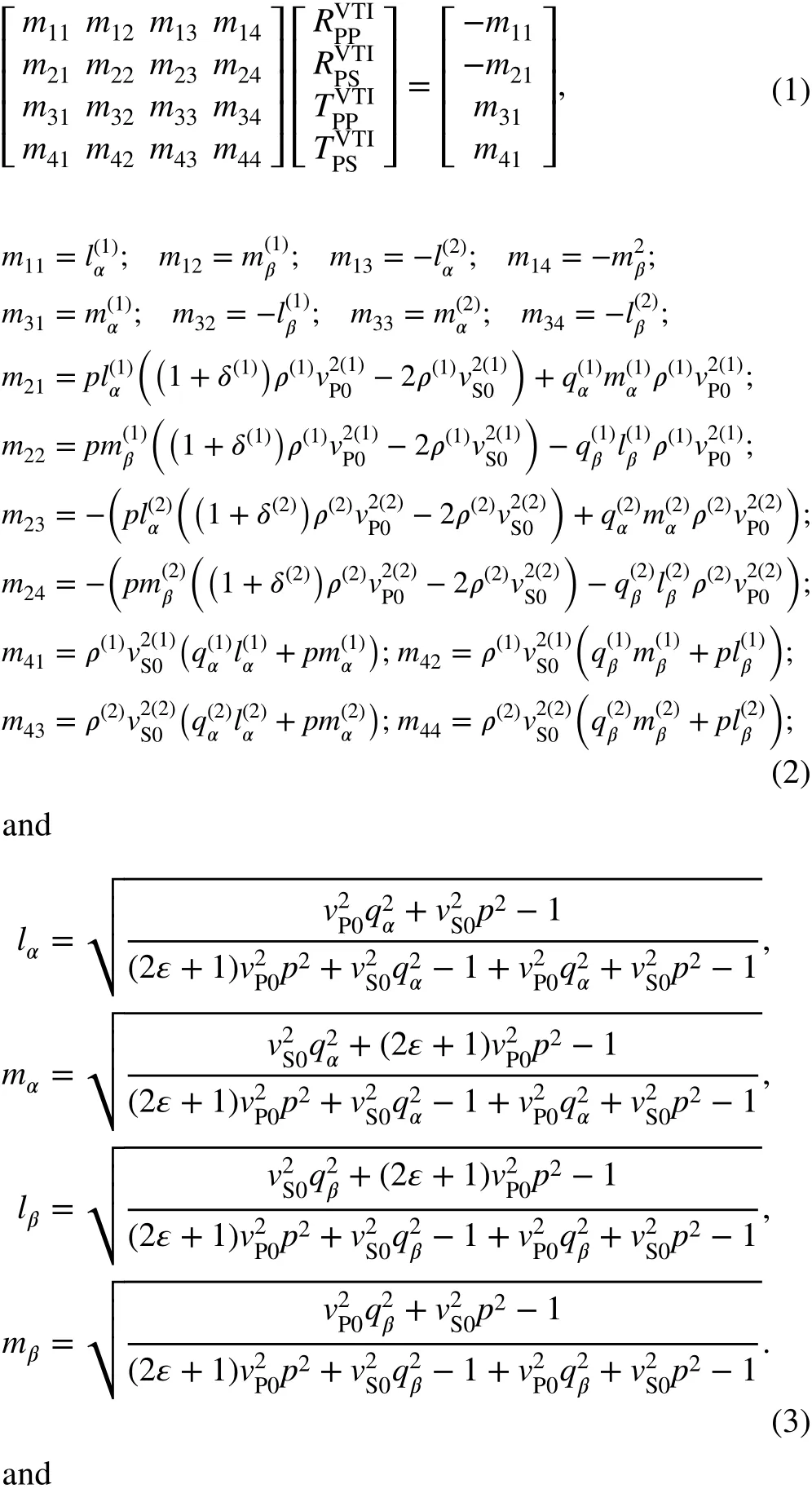
whereqαandqβare the vertical slownesses of the plane P-wave and the corresponding SV-wave, respectively,ρis density,vP0is the vertical velocity of P-wave andvS0is the vertical velocity of shear wave, andεandδare the anisotropy parameters.p=sin(θ)∕VP(θ)is the horizontal slowness,θis the phase angle, andVP(θ)is phase velocity of P-wave. In the above equations,αandβrepresent different wave modes, whereαrepresents the plane P-wave mode andβrepresents the corresponding SV-wave mode.

2.2 Deriving the new reduced approximation equations of VTI media

The exact expressions of the R- and T-coefficients of VTI media are very complicated. It is difficult to apply these equations to AVA analysis and inversion. When using the concept of GLI method to invert, we need to calculate the Jacobian matrix, and the complicated forms of the exact equations create a very complex problem and solution.Therefore, we first need to derive a new approximation formula before inversion. By analyzing the exact algebraic solutions of VTI media, we find that the expressions of the horizontal slowness and vertical slowness are complicated and have strong nonlinearity about the elastic parameters and anisotropy parameters. These directly cause the complicated structure of the exact equations of VTI media. Therefore,the strategy we adopt is to simplify the slownesses by ignoring the higher-order term that makes approximate equations more concise and straightforward. Then, they can be easily applied to AVA inversion.

The simpli fied horizontal slowness can be easily obtained according to the research results of Thomsen (1986). In VTI media, by assuming weak anisotropy, the phase velocity of P-wave can be linearized as follows:

According to Eq. (7), we can obtain the horizontal slowness with a relatively simpli fied form.

For the vertical slownesses, we use a new method to simplify them, and the derivation is given in “Appendix 1”.Then, the vertical slownesses in relatively simpli fied forms can be obtained by ignoring the higher-order term of two Thomsen anisotropy parameters, and their expressions are as follows:

Actually, the vertical slowness approximation is a linearization of the exact expression in Thomsen (1986) parameters. It greatly simpli fies the expressions of the R- and T-coefficients of VTI media. Equation (1) is an equation for the re flection/transmission coefficients. Equations (2), (3),(8) and (9) are the explicit expressions of the intermediate variables. Combining the above-mentioned equations,the forward operator (reduced equations) of the proposed method is obtained.

Table 1 Parameters of model 1: the VTI/isotropy interface (Rüger 1996)

Shale and sand interface models are then used to determine the calculation accuracy of the reduced equations.Tables 1 and 2 are the given model parameters. In model 1 (Rüger 1996), the lower sandstone is isotropic, and the upper shale has strong VTI anisotropy. In model 2, the layers are the Taylor sandstone and Mesaverde mudshale from Thomsen (1986), both of which have VTI anisotropy, and the interface has a strong impedance contrast.

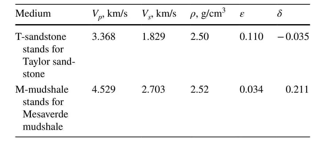
Table 2 Parameters of model 2: the VTI/VTI interface (Thomsen 1986)

Figures 1 and 2 show the comparison among the exact solutions and corresponding approximations of the re flection coefficients of VTI media for both models within a P-wave incidence range of 0°–60°. Figures 1 and 2a, b show the comparison of P-wave re flection coefficients and the comparison of S-wave re flection coefficients, respectively.Although the weak anisotropy assumption was meant to simplify the processing of the horizontal slowness and vertical slownesses, the re flection coefficients calculated by the new reduced approximation equations have satisfactory calculation accuracy at a strongly anisotropic interface, especially for P-wave. This ensures the accuracy of the inversion results(as can be seen from these figures).

2.3 Analysis of the linearity and uniqueness of the inversion

The linearity and uniqueness of the inversion problem are investigated by using RFMs. For a nonlinear function, if the RFMs show closed contours with one minimum, the nonlinear function can be successfully applied to inversion by using the GLI method with a second-order Taylor series expansion (Macdonald et al. 1987; Demirbag et al. 1993;Larsen 1999; Kurt 2007). The residual error function for theRPPdata set is given below (Larsen 1999):

whereRjm−ppis the re flection coefficient calculation result of P-wave for a chosen set of model parameters (RPPvalues from the new reduced equations) andjis angle.(m,n)is the calculation result of the same equation to different values of the chosen input parameter pair(m,n), andLis the critical incident angle.

Fig. 1 Comparison of the exact re flection coefficients equations (solid line), Rüger approximate equations (plus signs) and reduced re flection coefficients equations (circles) for model 1. a P-wave re flection coefficients, b S-wave re flection coefficients

Fig. 2 Comparison of the exact re flection coefficients equations (solid line), Rüger approximate equations (plus signs) and reduced re flection coefficient equations (circles) for model 2. a P-wave re flection coefficients, b S-wave re flection coefficients

According to the model parameters in Table 2, the corresponding RFMs figures for the 45 parameter pairs, composed of ten parameters of the new reduced equations, can be obtained. When calculating the residual error, the maximum incident angle is 47° which is the critical angle for the case of a PP re flection. There are 45 RFMs for all parameter pairs, which are too many for one paper to present thoroughly. By analyzing these RFMs through direct observation to determine whether they show closed contour with single minimum, it is seen that all RFM figures are smooth and regular. Also, most of them show closed contours around the actual parameters, indicating that GLI inversion and Marquardt inversion methods are applicable (Macdonald et al.1987). Furthermore, we should also note that the RFMs forparameter pairs for the reduced equations do not show closed contours around the true parameters. The RFMs for PP re flections show non-uniqueness for inversion of these pairs, and if we simply use the GLI method to find the minimum of the inversion problem, it may be unstable and inaccurate(Macdonald et al. 1987; Larsen 1999). Actually, Demirbag et al. (1993) and Larsen (1999) analyzed the RFMs of the exact Zoeppritz equations, and the RFMs forandparameter pairs for PP re flections also do not show closed contours around the true parameters. Even when using both PP and PS re flection data, the RFM forstill does not have closed contours. However, Lu et al. (2015)linearized the Zoeppritz equations by using the two-term Taylor series expansion and performed nonlinear joint inversion by using the Levenberg–Marquardt method. The process still gave high-resolution inversion results. Based on Bayesian theorem, Zhou et al. (2017a, b) achieved nonlinear inversion based the Zoeppritz equations by combining the concept of GLI inversion and IRLS algorithm. Both the P-wave inversion and joint P- and S-wave inversion can have accurate inversion results. The previous research suggests that as long as the RFMs are regular, nonlinear equations can be linearized using a two-term Taylor series expansion and then can be applied to the inversion successfully after introducing a regularization constraint. In addition, Macdonald et al. (1987) and Downton and Lines (2001) in their studies pointed out that prior information of estimated parameters is usually assumed to obey a speci fic distribution, can be introduced by using Bayesian theorem to construct an objective function. This can effectively decrease the uncertainty of nonlinear inversion algorithm and enhance the inversion accuracy. It can be seen from the above analysis that the nonlinear inversion objective function constructed by using the new reduced approximate equations can be solved stably.

Fig. 3 Residual function maps of model 2 fo (left) and(right) parameter pairs. Only rdata set was used to produce the PP residual errors. Contour values change from 0.001 to 0.01 by increments of 0.001. The black dot in all figures indicates actual values of the model parameters. Subscript 1 indicates the upper medium, and Subscript 2 indicates the lower medium

2.4 Prestack AVA inversion

Combined seismic data and prior information can be integrated into the Bayesian inversion theory framework and has been widely used in seismic inversion and other algorithms(Buland and Omre 2003; Rabben et al. 2008; Alemie and Sacchi 2011; Bachrach 2015; Zhou et al. (2017a, b); Wu et al. 2014; Jin et al. 2017, 2018). When using Bayesian theorem to construct an objective function, the likelihood function of the data can be expressed:where g is the forward operator, andrepresents the model parameters vector whereA,B,C,DandE are interested parameters (two vertical velocities, density and two Thomsen anisotropic parameters; each of them is a vector withNelements, andNis the size of model parameters).The matrixCDis the noise covariance matrix, andNdis the length of the seismic data.

For multi-mode joint inversion, Eq. (11) can be extended to the following form (Zhou et al. 2017a):

Shale reservoirs typically have strong VTI anisotropy,which leads to a clear interface with the surrounding layers. In order to enforce the sharp layer boundaries in the vertical direction seen in these reservoirs, a targeted reasonable prior model should be introduced. Theune et al.(2010) pointed out that the blocky inversion algorithm based on Bayesian theory could effectively enhance layer boundaries in prestack AVO/AVA inversions. The Laplace constraint has been suggested to perform more reliably compared to other prior models. Therefore, the prior model is composed of two parts: (1) background prior model (a Gaussian term containing the prior low-frequency trend and statistical correlation among the model parameters;and (2) a blockiness constraint term with heavy tails.

First, assuming the model parameters follow the Gaussian distribution,

The blockiness constraint is then introduced to enhance sparseness in the vertical direction. Ignoring normalization constants, we can obtain the following expression:

where Cmis a block diagonal matrix containing the statistical correlations information between different parameters,μis the mean vector of the model parameters (one for each model parameter),D is a first-order differential matrix, and thekl,l=1,2,3,4,5parameters are scaling parameters that can be different for each of model parameters. Generally,these scaling parameters can be obtained from logging data by utilizing a maximum likelihood estimator (MLE) (Theune et al. 2010).

Substituting Eqs. (12) and (14) into Bayesian theory(Ulrych et al. 2001), the inversion problem can be converted into a problem that solves the minimum value of the objective function (J1(m)):

Generally, the noise terms and the observed seismic data are assumed to be uncorrelated, so that the matrix CDcan be reduced to a diagonal matrix. Then, the matrixCDcan be expressed as,CD=I, whereis the noise variance,and I is anNd×Ndidentity matrix. Assuming that the noise variances of the P- and S-wave data areand, respectively, Eq. (15) can be simpli fied to:

According to Zhou et al. (2017b), the minimum of Eq. (16) can be found by combining the concept of GLI method and the IRLS algorithm, providing:

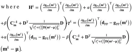
The derivation of the Jacobian matrixis given in “Appendix 1.” Ultimately,the updated iteration equation of the interested parameters is given by:

whereηkcontrols the step size ofkth iteration.

Fig. 4 True model data (solid line) and initial model data (dashed line)

Fig. 5 Synthetic prestack angle gathers (a) and synthetic prestack angle gathers with added random noise with S/N = 2 (b)

3 Synthetic data example

The model parameters shown in Fig. 4 are used to verify the feasibility and stability of the proposed method. In Fig. 4,the solid lines represent the curves of true elastic parameters and anisotropic parameters, and the dashed lines are the initial model data. In synthetic data example, the initial model can usually be obtained by smoothing the true data curve.The synthetic data are obtained by convolving the re flection coefficients calculated by the exact re flection coefficients equations of VTI media with a Ricker wavelet (the main frequency is 30 Hz), which are directly the prestack angle gathers. The synthetic data consist of ten traces with angle range of 4°–40°. In order to observe the noise suppression performance of the proposed method, random noise with a signal-to-noise ratio of 2 was added to the synthetic data.TheS/Nwas de fined by the root-mean-square amplitude.These synthetic prestack angle gathers we mentioned above are shown in Fig. 5.

Table 3 Correlation coefficient between the inversion results and the true values

For the synthetic PP angle gathers without noise (Fig. 5a),the following inversion methods were implemented: (1)P-wave data inversion by using the proposed method; (2)P-wave data inversion by using Rüger linear approximate formula; (3) joint P- and S-wave inversion by using the proposed method; (4) joint P- and S-wave inversion by using Rüger linear approximate formulas. Then, the correlation coefficients between the inversion results and the real values are calculated and shown in Table 3. Figure 6a, b shows the inversion results of the proposed method and the inversion method based on Rüger linear approximate formula, respectively. From the comparison of the proposed method versus the Rüger linear approximate formula inversion results and Table 3, we can see that when there is no noise, the inversion accuracy of the proposed method is much greater than that of the method based on the Rüger approximate formula. In theory, joint P-and S-wave inversion can enhance the stability of the inversion and improve the accuracy of inversion results due to the introduction of the converted wave information. However, if the formulas of S-wave re flection coefficients used for the joint inversion have large calculation errors, the accuracy improvement of joint inversion will be greatly diminished and the applicability of joint inversion will be limited. From the comparison of Fig. 6a, c and Table 3, the joint inversion by the proposed method further improved the accuracy of the inversion results. Comparing Fig. 6b, d, the joint inversion based on Rüger linear approximate formulas cannot enhance the obtained accuracy of the interested parameters under the condition of the model parameters shown in Fig. 4 because of the low calculation accuracy of Rüger’s S-converted wave re flection coefficients formula.

In order to observe the noise suppression performance of the proposed method, the P-wave inversion and joint P- and S-wave inversion are implemented by using the noisy data(Fig. 5b). The corresponding inversion results and the correlation coefficients between the true values and the inversion results are shown in Fig. 7 and Table 4, respectively. The three elastic parameters and two anisotropic parameters were accurately estimated, even whenS/N= 2, and the accuracy of the inversion results can be further improved by the joint inversion. To sum up, the proposed inversion method can reasonably estimate the five VTI parameters from the prestack seismic data while remaining stable. Moreover, the inversion accuracy of the proposed method is much higher than that of the inversion method based on the Rüger linear approximation formulas.

4 Field data example

The P-wave data were the only data used for inversion test because S-wave data were not collected. Figure 8 shows the actual angle gather with a sampling interval of 2 ms at the location of Well A with an effective angle range of 3°–45°(1° intervals), all of which were used in the inversion process. The wavelets used in the inversion are angle-independent wavelets estimated from well logs and angle gathers.According to the quality of the actual data, all incidence angles were divided into five segments, and each segment estimated one wavelet (Fig. 9). The data have been processed by a series of conventional processing procedures, such as amplitude compensation and correction, deconvolution,noise suppression, NMO, interbedded multiple suppression processing and prestack time migration.

Fig. 6 Inversion results. The black line indicates the initial model data, the blue dotted line indicates the inversion result, and the red line indicates the true model data. a P-wave data inversion by using the proposed method, b P-wave data inversion by using the Rüger linear approximate formula, c joint P- and S-wave inversion by using the proposed method, d joint P- and S-wave inversion by using the Rüger linear approximate formulas

In Fig. 10, the curves of anisotropy parametersεandδare estimated based on the existing anisotropy rock physics model by using logs of volumetric fraction of clay and other brittle minerals (Zhang et al. 2014). Figure 10a shows the inversion results by using the proposed method.The curves of the inversion results correspond to the well with logging curves, indicating that the proposed method is valid and feasible in application to field data. Based on these inversion results, the synthetic angle gather and residual wave fields between the field data and synthetic angle gather were obtained, and are shown in Fig. 8. There is still some effective amplitude in the residual due to the in fluence of the actual data quality. We also used the Rüger linear approximate formula for the same inversion (Fig. 10b).The proposed inversion method can signi ficantly improve the accuracy of inversion results, especially for anisotropy parameters and compared to the Rüger formula (Fig. 10a, b).The proposed method based on the reduced approximation equations can estimate the elastic parameters and anisotropy parameters of VTI media formations with high accuracy,which will greatly aid in the exploration and development of shale reservoirs.

Fig. 7 Inversion results by using the proposed method (S/N = 2). a P-wave inversion, b Joint P- and S-wave inversion

5 Discussion

Existing approximate formulas of VTI media re flection coefficients all have similar forms. Although the forms of these approximation formulas are very simple, they all have the same problems of low calculation accuracy and poor applicability. Moreover, the exact algebraic solution has very complicated form and strong nonlinearity, creating an algorithm that is impractical in field applications. These problems also greatly limit the accuracy of AVA inversion in VTI media. Compared with the exact equations, the slowness equations of the new derived reduced approximation equations proposed here have a relatively simple form,while ensuring that the new reduced equations retain the high calculation accuracy. These equations can better handle the above-mentioned problems. When using RFMs to analyze the linearity of the reduced equations, we only usedRPPdata to compute residual errors. In actuality, when using bothRPPandRPSdata to compute the residual errors, the size of the closed contours becomes smaller and the RFM forparameter pairs also shows closed contours around the true parameters. This shows that joint inversion is able to decrease the ambiguity of the estimation results.In the theoretical derivation part, the proposed method has been extended to multi-mode joint inversion. However, if we want to use the joint inversion to improve the stability and accuracy of the inversion results, the precondition assumption that multi-wave data are well-matched in the time domain should be guaranteed.

Table 4 Correlation coefficient between the inversion results and the true values (S/N = 2)

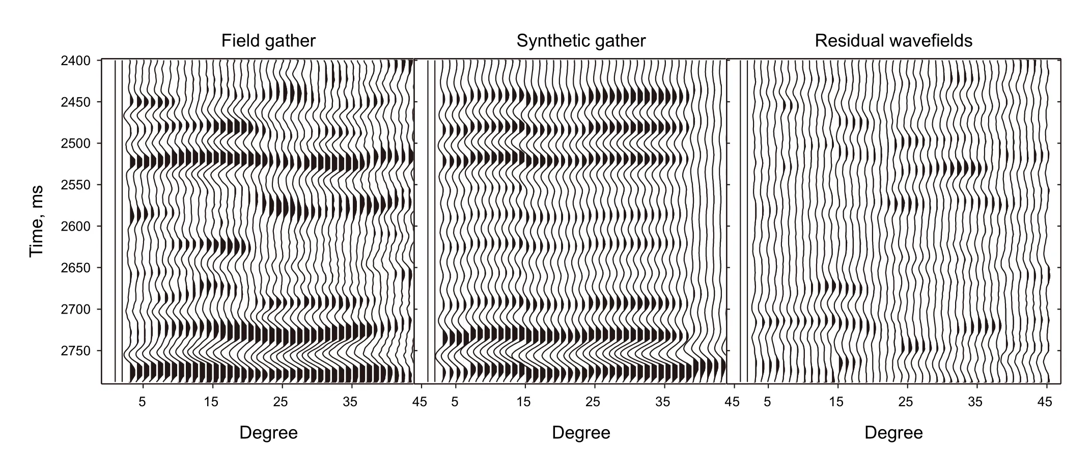
Fig. 8 Input field gather (left), synthetic angle gather (middle), and residual (right) between the input and the synthetic gather at the location of well A

Fig. 9 Estimated angle-independent wavelets used in inversion

6 Conclusion

In this paper, we derived a set of new nonlinear approximate equations with relatively simple form by starting from the exact re flection coefficients equations of VTI medium and ignoring the higher-order term. These reduced equations retain sufficient calculation accuracy, especially for P-wave re flection coefficients and for field data inversion.The inversion objective function was then constructed by combining the reduced equations and Bayesian theory. Furthermore, the blockiness constraint which followed the differentiable Laplace distribution was added to the prior model in order to improve the contrasts between layers. This can effectively improve the adaptability and accuracy of the VTI media prestack AVA inversion. The RFMs analysis results of the reduced equations show that the minimum of the objective function can be steadily obtained by combining the concept of the GLI method and the IRLS algorithm. The iterative updating equation of the VTI parameters can be obtained, and the nonlinear estimate of these parameters can be achieved. The examples demonstrated that the proposed method can not only accurately invert the VTI parameters of the reservoir, but also is obviously better than the method based on Rüger approximate formulas.

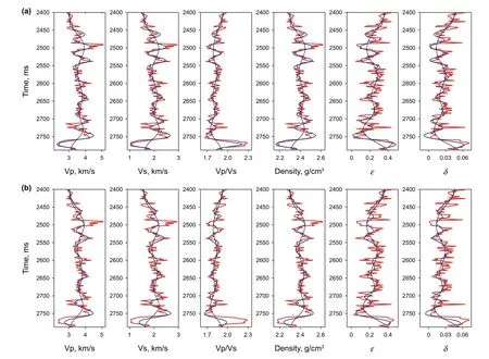
Fig. 10 Comparison of the logging data and inverted result at the well location. The black line indicates the initial model, the blue line indicates the inversion results and the red line indicates the logging data. a Proposed method, b Rüger linear approximate formula

Open AccessThis article is licensed under a Creative Commons Attribution 4.0 International License, which permits use, sharing, adaptation, distribution and reproduction in any medium or format, as long as you give appropriate credit to the original author(s) and the source,provide a link to the Creative Commons licence, and indicate if changes were made. The images or other third party material in this article are included in the article’s Creative Commons licence, unless indicated otherwise in a credit line to the material. If material is not included in the article’s Creative Commons licence and your intended use is not permitted by statutory regulation or exceeds the permitted use, you will need to obtain permission directly from the copyright holder. To view a copy of this licence, visit http://creat iveco mmons.org/licen ses/by/4.0/.

Appendix 1

Substituting the Thomsen anisotropy parameters into the vertical slownesses, we have:

Simplify the above formulas:

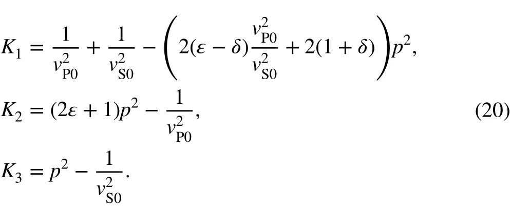
SubstitutingK2andK3intoK1, we have:

Then ignoring the higher-order termthe following expression is acquired:

Then ignoring higher-order termsandthe following expression is acquired.

Assuming that

the following expression is acquired.

T h e n a d d i n g h i g h e r-o r d e r t e r m s, the following expression is acquired

By substituting Eq. (25) into Eq. (27), we have:

By substitutingK1and Eq. (28) into the exact expressions of vertical slownesses, we have:

Appendix 2

The Jacobian matrix can be written as:

whereW is the wavelet matrix, and rpp(m)and rps(m)represent the P-wave re flection coefficients sequence and converted S-wave re flection coefficients sequence, respectively.

For a certain angleθi, we have:

Extending Eq. (31) to thenth incident angles situation,the Jacobian matrix will become a (n×N)×5Nmatrix, and then it will be extended to the situation of joint P- and S-wave inversion. Ultimately, the Jacobian matrixbecomes a (2n×N)×5Nmatrix.

The new reduced equations of re flection and transmission coefficients of VTI media can be represented in matrix form via the following expression.

The derivative of both sides of Eq. (37) with respect to the elastic parameters and anisotropic parameters is given by:

Then, the first-order partial derivative of the R- and T-coefficient of the interface with respect to the ten unknown parameters contained in the reduced equation can be obtained.

Eventually, by combining the above derivation, we can obtain the first-order partial derivative of the forward operator with respect to model parameters (Jacobian matrix).