Investigation of Influence Coefficient Method for Flutter Analysis*

Wei Liu Xiu-quan Huang ,2 Ding-x i Wang ,2 Ruo-yang Liu

(1.School of Power and Energy,Northwestern Polytechnical University,Xi’an,China，Email:xiu quan_huang@nwpu.edn.cn;2.Shaanxi Key Laboratory of Internal Aerodynamics in Aero-engines,Northwestern Polytechnical University,xi'an,China;3.Aero Engine Academy of China,Beijing,China)

Abstract： Influence coefficient method has long been used for both numerical and experimental flutter investigation. In an experimental investigation, quite often a linear cascade or an annular cascade sector with 3～11 blades is used with tail boards at the upper and lower ends.The middle blade only is driven to vibrate and the generated unsteady pressure on all the blades are measured to construct the unsteady pressure for a traveling wave vibration mode using the influence coefficient method. When using the influence coefficient method in a numerical analysis,there is no need to use the tail boards,and periodic boundary condition can be applied to ensure the flow periodicity.Some point out that 9 or even 11 blades are necessary to obtain results which are independent of the number of blades being used.This article investigates the effects of blade count,Mach number and position of the vibrating blade on analysis results by using the harmonic balance method for unsteady flow field analysis. It is concluded that 7 blades with a periodic boundary condition and 13 blades with a tail board boundary condition are sufficient to get accurate results for the cascade under investigation.It is also revealed that the vibrating blade is best placed at the middle position.

Keywords：Influence Coefficient Method,Flutter,Linear Cascade,Travelling Wave Method

Nomenclature

Q conservative variables

vx,vθ,vrvelocity in the x direction, θ direction and r direction

ρ,p,E density,pressure and total internal energy

τ stress tensor

μ effective dynamic viscosity

n the number of harmonics

W worksum

T blade vibration period

Cp( N,0)the influence on blade N produced by blade 0 vibrating

σ inter blade phase angle the unsteady aerodynamic force on the

Cp,0reference blade surface

N blade index

1 Introduction

The development of high thrust-weight ratio aero-engines translates to the development of very compact and highly loaded turbomachinery. The consequence is that the unsteadiness of the flow field is enhanced, and the stiffness of blades is reduced. This inevitably intensifies the interaction between blades and their surrounding working fluid,leading to prominent flow induced vibration issues. Flutter belongs to the self-excited vibration pedigree and should be avoided entirely, as it can lead to high cycle fatigue or even quick blade failure during a component or engine test. To achieve blade design free from flutter, there is a need to assess blade flutter accurately and quickly in a daily design loop.To do this asks for accurate and fast numerical methods for analyzing blade flutter.

There are quite a few numerical methods with different level of fidelity for blade flutter analysis. Quite often time cost of those methods scales with their fidelity, with high fidelity methods being more time consuming. To date for design comparison in industrial environment, decoupled techniques based upon the energy method have been the choice.Two typical ones are the traveling wave method (TWM) and the influence coefficient method(ICM).

The TWM was proposed by Lane (1956)[1]. It is assumed that all the blades in a blade row are identical and vibrate at the same frequency and mode shape,but fixed phase difference between any two adjacent blades.In an experimental study, the method can be applied to annulus configurations only. Though the travelling wave vibration mode is a better representation of reality in contrast to the influence coefficient method, it is rarely used in an laboratory cascade test. This is because all blades have to be driven to vibrate,which is quite difficult. Particularly there is a need to maintain the fixed phase difference between adjacent blades and this has to be carried out for all possible inter blade phase angles separately. Nevetheless, the TWM has been widely used for numerical analyses. In a numerical flutter analysis, one blade passage is normally employed with the phase shift boundary condition being applied at the geometric periodic pairs.

The ICM was initially and has been widely used for experimental investigation of unsteady flow due to blade vibration, such as the work by Hanamura (1980)[2], Buffum and Fleeter (1990)[3], Frey and Fleeter (2001)[4]. It is assumed that the unsteady flow on a blade due to a traveling wave vibration mode is equal to the superimposition of the unsteady flow due to each blade vibration. The method can be employed in a linear cascade, an annulus cascade sector or a whole annulus configuration. In an experiment, one blade is driven to vibrate while unsteady flow on all blade surfaces are measured. Different from the TWM, there is no need to consider different inter blade phase angle.Unsteady flow corresponding to different inter blade phase angle is obtained through post-processing using the same set of data.With the assumption that the influence of one blade on other blades diminishes quickly in the pitch-wise direction, a limited number of blades can be employed in either a test or computational domain. For example,7 blades were used by Huang et al.(2006)[5], Yang et al.(2004) [6], Vogt et al (2007)[7] and Kven Hsu and Daniel Hoyniak (2013)[8]; Mårtensson et al(2005)[9] used only three blades to get accurate results for a no-tip-clearance model.

The ICM has also been used for numerical flutter analysis to reduce time cost. Waite and Kielb (2015)[10] used the ICM to study a low-pressure turbine flutter boundary and found that loading the blade can stabilize or destabilize the blade depending on the mode shape. Kielb et al (2007) [11]used the ICM to describe how to model the aerodynamically mistuned turbomachinery. Nenad Glodic and Damian Vogt(2011)[12]investigated mistuning with the ICM by using experimental and numerical simulation to yield travelling wave mode results and found that mistuning can lead to a measurable even though only moderate change in aeroelastic stability.

Compared with the TWM, the ICM has some advantages and shortcomings. K Vogel et al (2017)[13] compared the ICM with the TWM based on an axial turbine and a centrifugal compressor using a frequency domain method in numerical simulation and identified some differences according to the results of two methods.The TWM needs to repeat experiment at different IBPAs and vibrate all blades in experiment.Conversely, the ICM does not need to repeat experiment for changing IBPA but need to measure unsteady response(influence coefficient) on all blades. The ideal model should contain all blades of one row, but the cost is too high, and it is unnecessary if the unsteady response decays rapidly with the increase of the pitch wise distance. So, choosing a suitable model without too many blades can effectively reduce cost.Thus, how to choose a model in different cases is the key to use the ICM efficiently. In addition, the ICM also has some other questions to be answered regarding its application,such as positioning of the vibrating blade, its validity in a transonic flow.

The linear turbine cascade of Durham University which was developed by Huang(2006)[5]is used to carry out investigation to answer the questions mentioned above.Compared with the previous research by Campobasso (2004)[14] who used the linear harmonic method,the harmonic balance method put forward by Hall and Thomas (2002)[15] is applied in this paper.Furthermore,in a linear cascade experiment,in order to have a good flow periodicity,it is essential to place upper and lower tail boards. These tail boards are not required in numerical simulation. This paper also investigates the effect of tail boards on flow field.

2 Numerical Methods

All the simulations in this paper are performed using the in-house flow solver-Turbo3D of which the details can be found in the paper by Huang and Wang(2016)[16].

This code solves the Reynolds-averaged Navier-Stokes equations.The JST scheme is used for convective flux terms.For viscous terms, spatial gradient of primitive variables is acquired based on a cell central Gauss integration. Explicit and implicit hybrid methods are used for time marching: the five stage Runge- Kutta method and the LUSGS method which is used for residual smoothing. In order to accelerate convergence further, the local time step and multigrid methods are used in the program.

For time periodic unsteady flow simulations, the harmonic balance method is the choice which represents a temporal periodic unsteady flow solution using truncated Fourier series.The number of harmonics can be set a priori and more harmonics means higher accuracy but more time cost.To resolve n harmonics,the unsteady N-S equations are solved for at least 2n+1 time instants simultaneously. The solutions at the 2n+1 time instants can be used to obtain the Fourier coefficients using Fourier transform. Then the Fourier coefficients can be used to calculate the time derivative term of the unsteady equation. In this way, the N-S unsteady equations are converted to 2n+1 sets of quasi steady equations. Compared with the time domain method, it can reduce lots of computing time.

2.1 Calculation of Worksum

Worksum is work done by the unsteady fluid force on a blade during one vibrating period. It is an indicatorr for flutter prediction. If the worksum is positive, flutter may occur.It can be calculated in this way: the unsteady aerodynamic force at each point on a blade surface is multiplied by the velocity of the point and integrated over the entire blade surface in one vibration period.The formula is as follows:

where T is the vibration period, A is the blade surface, p is the pressure, n→is the blade surface normal vector,and u→is the velocity vector of a point on a blade surface due to blade vibration.

2.2 Influence Coefficient Method(ICM)

The ICM obtains the aerodynamic influence on its own and other blades by vibrating a reference blade in a row. For example,for a cascade model with 7 blades as shown in Figure 1, the middle blade has an index of 0 and blades right to it have positive indices and blades left to it have negative indices. The measured unsteady aerodynamic force coefficient on blade N includes the amplitude and phase angle and is represented using a complex number Cp(O,N). The unsteady force coefficient on the reference blade when all blades vibrate with an inter blade phase angle of σ can be obtained as follows

where 2M+1 denotes the number of blades being used, σ is the inter blade phase angle. When σ is positive, it means blade N has a phase lead with respect to blade 0. Now we can see that we can get the unsteady aerodynamic force coefficient for any inter blade phase angle with the known Cp(O,N) which is only calculated once.This is the advantage of the ICM compared with the TWM.

Fig.1 Blade index in a cascade

2.3 Traveling Wave Method(TWM)

The TWM is also an effective method for calculating the unsteady force due to blade vibration. The TWM and ICM both assume that all blades vibrate with the same mode shape and frequency but a fixed phase difference between adjacent blades called inter blade phase angle. Compared with the ICM, the TWM has an advantage that it only needs one passage for the computational domain. But the TWM needs to repeat the simulation for each IBPA to get a worksum-IBPA curve.

2.4 Test Case

The Durham linear turbine cascade is chosen as the test case which was developed by Huang (2006)[5].The cascade consists of 7 prismatic turbine blades, upper and lower tail boards and other experimental devices as shown in Figure 2.

For numerical simulation, a H-type structured mesh is used. For the axial, circumferential and radial directions,there are 225 65 and 65 points respectively.There are in total 950 625 points in a single blade passage. The blade surface mesh is shown in Figure 3(a).

To obtain unsteady flow field, the middle blade of the cascade is driven to vibrate at a first bending mode. The mode shape is shown in the Figure 3(b).The vibrating amplitude distribution varies from tip to hub linearly. The amplitude at the tip is 2.6mm, and that at the hub is 0.4 mm. The vibration frequency of the blade is set to 21.245Hz and the corresponding reduced frequency is 0.2.

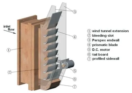
Fig.2 Durham linear turbine cascade model with tail boards

Fig.3 The blade surface mesh and the axial component of blade mode shape of the test case

3 Results and Discussions

A series of simulations are performed to study the application of the ICM to flutter analysis. The results are divided into three sections below: First, results obtained using the ICM are compared with the experimental data and those from the TWM to validate the accuracy of the ICM. Second,at a low Mach number condition, investigation is carried out to study the effect of the number of blades on aerodamping calculation when the periodic boundary condition or the tail boards are imposed at the upper and lower boundaries.When the tail boards are used, the effects of discarding data from blades adjacent to tail boards and the position of the vibrating blade on aerodamping calculation are also investigated.Third, similar investigation is carried at a higher Mach number to study the effect of the number of blades on aerodamping calculation for both periodic boundary conditions and tail board boundary conditions and the effect of discarding data from blades adjacent to tail boards on aerodamping calculation.

3.1 Validation of ICM

In order to validate the accuracy of damping prediction using the ICM, the unsteady flow field obtained using influence coefficients in the numerical simulation are compared with the experiment data at a low Mach number condition.We performed two cases for the validation purpose. One case is that the computational domain consists of 13 blades with direct periodic boundary condition being applied at the upper and lower geometric boundaries.The other is to truely represent the test cascade. Hence the computational domain consists of 7 blades with tail boards being applied at the upper and lower geometric boundaries.For the low Mach number condition, the inlet total pressure is set to 107 000Pa, the inlet total temperature is set to 293K and the outlet static pressure is set to 101 325Pa.The flow direction at the inlet is axial. The inlet Mach number is about 0.1 and the highest Mach number in the flow field is about 0.3.

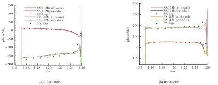
Fig.5 Comparison of the phase angle of the first harmonic pressure between the numerical simulation and the experiment data for a low Mach number condition(50%span)

Show in Figure 4 and Figure 5 are the amplitude and phase angle of the first harmonic pressure for two different inter blade phase angles (108 degrees and-90 degrees). In these figures, ICM (periodic) means the analyses using periodic boundaries and ICM (tailboard) means the analyses using tail board boundaries.The two set numerical results are both in good agreement with the test data.

The comparisons of damping coefficient between three numerical simulations and the experimental data are shown in Figure 6. Particularly, we calculate the damping coefficient for the case with tail board boundaries only using data from the middle three blades to be consistent with the test data processing.There are some differences between the numerical results and the experimental data,but the ICM results are in close agreement with the TWM results. The discrepancy can be due to the low resolution of the test data and investigation is being undertaken to look at this.

3.2 Results for Low Mach Number Condition

At the low Mach number condition, the inlet total pressure is set to 107 000Pa, the inlet total temperature is set to 293K,the inlet flow angle is set to be axial and the outlet static pressure is set to 101 325 Pa. Figure 7 and Figure 8 show the flow field from an steady analysis using a computational domain consisting of 7 blades with tail boards being imposed on the upper and lower boundaries.The tail boards are adjusted to make the pressure distributions as close as possible on different blades of the cascade model. The inlet Mach number is about 0.1, and the highest Mach number in the flow field is just 0.3.

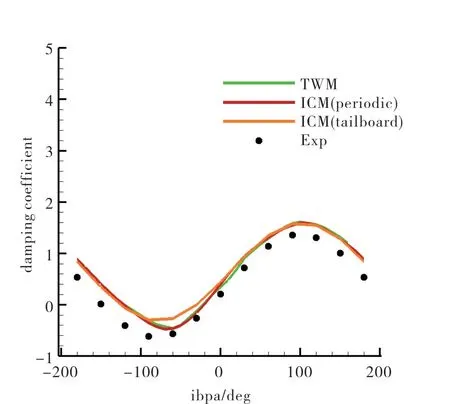
Fig.6 Comparison of the damping coefficient between the experiment data and the numerical simulation using the ICM and the TWM

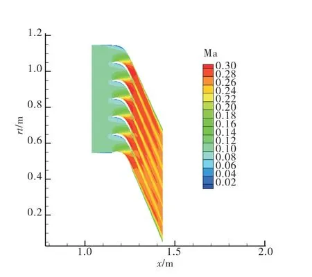
Fig.7 The Mach number contour at 50% span for the low Mach number condition

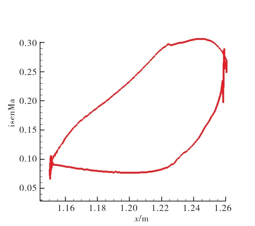
Fig.8 The Isentropic Mach number distribution at 50% span for the low Mach number condition

3.2.1 Effect of the number of blades on aerodamping when periodic boundary is applied

Investigation of effect of the number of blades used in a computational domain on aerodamping calculation when the periodic boundary condition is imposed on the upper and lower boundaries is presented in this section. Calculations are performed for domains consisting of 5, 7, 9, 11 and 13 blades, corresponding to 4, 6, 8 and 10 blade passages between the upper and lower boundaries.

Figure 9(a) displays the influence coefficients (IC) of each blade on the middle vibrating blade. In the figure, the number denotes the number of blades being included in a computational domain.It can be seen that the vibrating blade itself has the greatest influence, while the adjacent two blades have the second largest influence. The influence of other blades diminishes dramatically when they are away from the middle vibrating blade. The influence coefficients are asymmetric about the middle blade: the influence coefficient from blade-1 (on the pressure side of the vibrating blade) is greater than that from blade 1 (on the suction side of the vibrating blade).

Figure 9(b) shows the worksum-curves obtained using the ICM for domains with different number of blade passages.When the number of blades exceeds 5,the obtained worksum does not vary with the increase of the number of blades.That means it is unnecessary to include too many blade passages in a domain when the ICM method is used. For this particular case, 7 blades are sufficient to get results independent of the number of blade passages.

3.2.2 Effect of the number of blades on aerodamping when tail board boundary is applied

Tail boards have to be used in an experimental investigation employing a linear cascade.Quite often 7 to 9 blades are used in an experimental setup to reduce operation cost. In our investigation,analyses using a domain consisting of 6,8,10 and 12 blade passages are performed to calculate the worksum with results being shown in Figure 10. The worksum obtained from analysis using a domain consisting of 13 blades with periodic boundary condition being imposed on the upper and lower boundaries is also shown in the figure as the reference. Different from the analysis with the periodic boundary condition, the worksum obtained using 7 blades shows big difference from the reference. To get good agreement with the reference curve, the number of blades has to be increased up to at least 13.

The influence coefficients for different analyses are shown in Figure 10(a), different from Figure 9(a) the influence coefficients vary greatly with the number of blade passages. This indicates that the tail boards have great effect on the influence coefficients of every blades.

3.2.3 Effect of discarding data from blades next to tail board boundaries

From the previous section, it is recognized that the tail boards have great influence on influence coefficients and worksum,and this influence must be stronger on blades closer to the tail boards. Without extra analyses, we perform worksum calculation by discarding data from blades close to the tail boards for two analyses employing 11 blades and 13 blades. Figure 11(a) shows the obtained worksum using data from the middle 3,5 and 7 blades for a domain consisting of 11 blades or 10 passages, and Figure 11(b) shows corresponding data for a domain consisting of 13 blades or 12 passages. In the two figures, the reference refers to results obtained from an analysis using 12 blade passages with periodic boundary conditions. As can be seen from the above figures,there is a need to include at least 5 blades for this particular case when calculating the worksum and including data from blades next to the tailboards does not seem to have adverse impact on the worksum.

3.2.4 Effect of the vibrating blade position on aerodamping when tail board boundary is applied

Fig.9 Influence coefficients and worksum for the low Mach condition with periodic boundary conditions

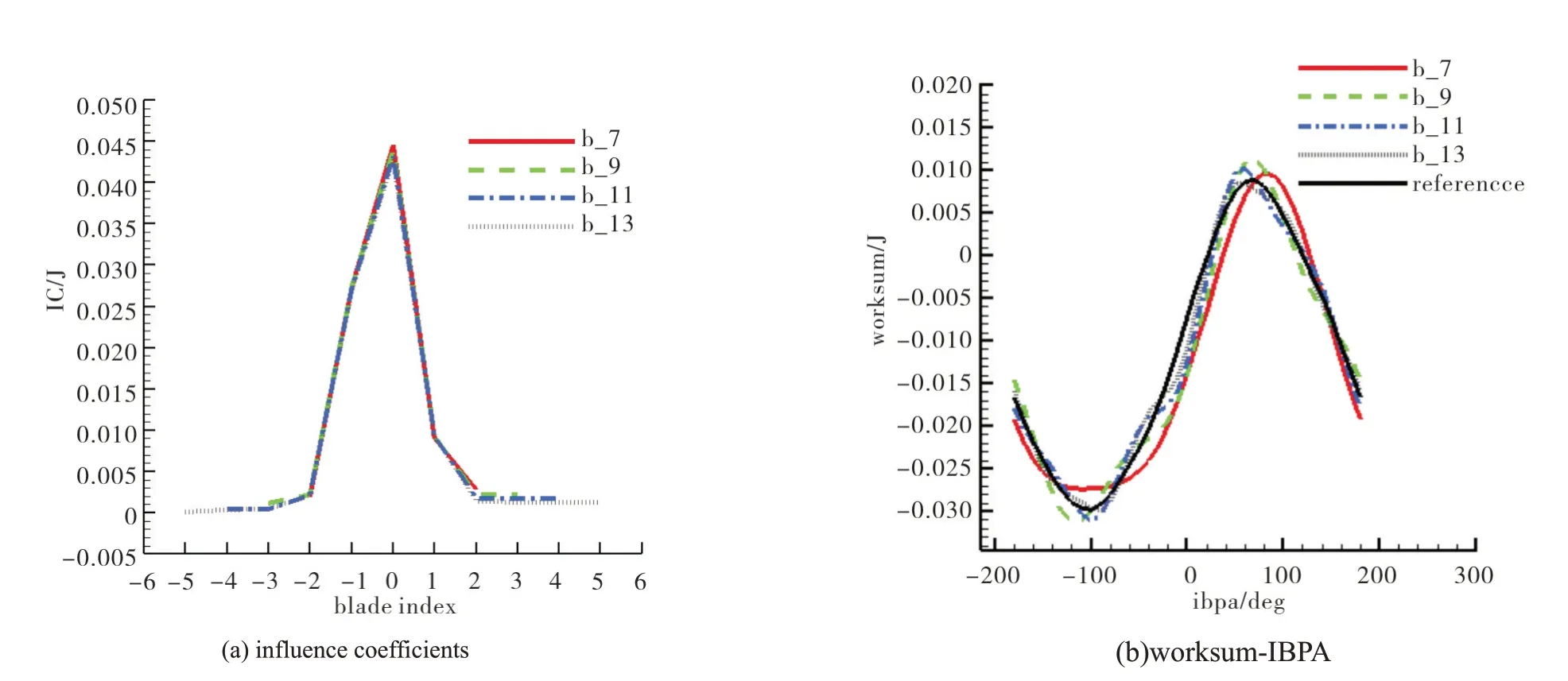
Fig.10 Influence coefficients and worksum for the low Mach condition with tail board boundary conditions

It is clearly from the figure that the influence coefficients are asymmetric about the middle blade, the influence coefficients on blades at its pressure side(particularly blade-1)are greater than those on blades at its suction side(particulary blade 1). Therefore, it is possible to set the vibrating blade away from the middle to achieve better results. We want to investigate how worksum varies if the vibrating blade is offset from the middle position by 1-3 blades toward the upper tail board or the lower tail board. Analyses were performed for one case consisting of 11 blades with different vibrating blade positions ranging from-3 to +3. Damping prediction results are shown in Figure 12. Again, the reference refers to results obtained from an analysis using 13 blades with periodic boundaries.

It can be seen from the Figure 12 that the influence of the vibrating blade position on worksum calculation is significant and offsetting it from the middle position has adverse effect on the calculated worksum. Therefore, the best vibrating blade position is the middle blade position.

3.3 Results for High Mach Number Condition

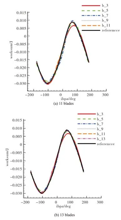
Fig.11 Effect of discarding data from blades close to tailboards on the calculated worksum

Fig.12 Difference situation of blades with offset.(11-blade)

Fig.13 Mach number contour at 50% span for the high Mach number condition

Fig.14 Isentropic Mach number distribution at 50% span for the high Mach number condition.

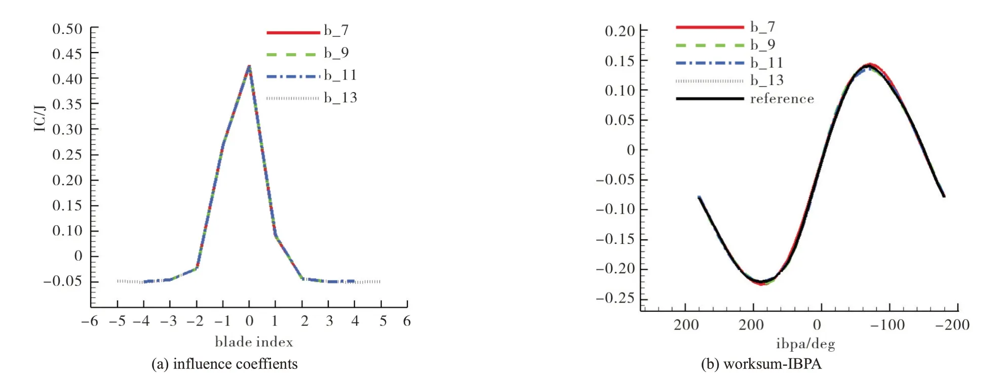
Fig.15 Influence coefficients and worksum obtained with different number of blades for the high Mach number condition and periodic boundary conditions

Fig.16 Influence coefficients and worksum for the high Mach number condition and tail board boundary conditions

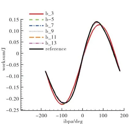
Fig.17 Effect of discarding data from blades close to tailboards on the calculated worksum(13-blade)

At the high inlet Mach number condition, the inlet total pressure is set to 187 000Pa, the inlet total temperature is set to 293 K,the inlet flow angle is set to be axial and the outlet back pressure is set to 101 325 Pa. Figure 13 and Figure 14 show the results from a steady analysis using a computational domain consisting of 7 blades with tail boards being imposed on the upper and lower boundaries. The inlet Mach number is about 0.3, and the highest Mach number in the flow field is 1.2.

3.3.1 Effect of the number of blades on aerodamping when periodic boundary is applied

Investigation of effect of the number of blades used in a computational domain on aerodamping calculation when the periodic boundary condition is imposed on the upper and lower boundaries is presented in this section. Calculations are performed for domains consisting of 5, 7, 9, 11 and 13 blades,corresponding to 4,6,8,10 and 12 blade passages between the upper and lower boundaries.

Figure 15(a) displays the influence coefficients of each blade on the middle vibrating blade.It can be seen that the vibrating blade has the greatest influence on itself, while the adjacent two blades have the second largest influence. The influence of other blades diminishes dramatically when they are away from the middle vibrating blade. The influence coefficients are asymmetric about the middle blade, the influence coefficients on blades at its pressure side are greater than those on blades at its suction side. This is the same as that for a low Mach number condition.

Figure 15(b) shows the worksum-curves obtained using the ICM for domains with different number of blade passages.When the number of blades exceeds 5,the obtained worksum does not vary with the increase of the number of blades.That means it is unnecessary to include too many blade passages in a domain when the ICM method is used. For this particular case, 7 blades are sufficient to get results independent of the number of blade passages. This is also the same as that for a low Mach number condition.

3.3.2 Effect of the number of blades on aerodamping when tail board boundary is applied.

Tail boards have to be used in an experimental investigation employing a linear cascade. Quite often 7 to 9 blades are used in an experimental setup to reduce operation cost.In our investigation,analyses using a domain consisting of 6,8,10 and 12 blade passages are performed to calculate the worksum with results being shown in Figure 16. The worksum obtained from analysis using a domain consisting of 13 blades with periodic boundary condition being imposed on the upper and lower boundaries is also shown in the figure as the reference. Different from the analysis with the periodic boundary condition, the worksum obtained using 7 blades shows big difference from the reference. To get good agreement with the reference, the number of blades has to be increased up to at least 13 which is the exactly the same as that for a low Mach number condition.

The influence coefficients for different analyses are shown in Figure 16(a), different from Figure 15(a) the influence coefficients vary greatly with the number of blade passages. This indicates that the tail boards have great effect on the IC of every blade.

3.3.3 Effect of discarding data from blades next to tail board boundaries

From previous section, it is recognized that the tail boards have great influence on influence coefficients and worksum like the low Mach number condition.Without extra analyses, we perform worksum calculation by discarding data from blades close to the tail boards for one analysis employing 13 blades. Figure 17 shows the obtained worksum using data from the middle 3, 5 ,7 ,9 ,11 and 13 blades for a domain consisting of 13 blades or 12 passages. In the figure,the reference refers to results obtained from an analysis using 13 blades with periodic boundary conditions. As can be seen from the above figures, there is a need to include at least 5 blades for this particular case when calculating the worksum and including data from blades next to the tailboards does not seem to have adverse impact on the worksum.

4 Conclusions

In this paper,some simulations are performed to answer the questions of the ICM regarding its application. The unsteady flow field obtained using the ICM is compared with that of the TWM and the experiment data.The following conclusions can be drawn from the investigations:

For the low Mach number condition:

1) It can be said that the ICM has the same accuracy as the TWM,though there are some differences between the experimental data and the results of the two methods.

2)The influences of the vibrating blade offsets on worksum calculation are significant, but overall the vibrating blade offset cannot improve the damping prediction accuracy.

For both low and high Mach number conditions:

1) If the periodic boundary condition is imposed on the upper and lower boundaries, the prediction accuracy is guaranteed when the number of blades used in a computational domain is no fewer than 7.

2) The influence of the vibrating blade on blades at its pressure side is greater than that on blades at its suction side.

3)Tail boards which have to be used in an experimental investigation employing a linear cascade have a great effect on damping prediction. Compared with the periodic boundary conditions, to obtain aerodamping independent of the number of blades, the number of blades used in a computational domain has to be increased up to at least 13.

4) Discarding data from blades close to the tail boards can also affect the prediction accuracy.At least 5 blades need to be included when calculating the worksum for this cascade model.