Yield Stress Prediction Model of RAFM Steel Based on the Improved GDM-SA-SVR Algorithm

Sifan Long,Ming Zhao and Xinfu He

Abstract:With the development of society and the exhaustion of fossil energy,researcher need to identify new alternative energy sources.Nuclear energy is a very good choice,but the key to the successful application of nuclear technology is determined primarily by the behavior of nuclear materials in reactors.Therefore,we studied the radiation performance of the fusion material reduced activation ferritic/martensitic(RAFM)steel.The main novelty of this paper are the statistical analysis of RAFM steel data sets through related statistical analysis and the formula derivation of the gradient descent method(GDM)which combines the gradient descent search strategy of the Convex Optimization Theory to get the best value.Use GDM algorithm to upgrade the annealing stabilization process of simulated annealing algorithm.The yield stress performance of RAFM steel is successfully predicted by the hybrid model which is combined by simulated annealing(SA)with support vector machine(SVM)as the first time.The effect on yield stress by the main physical quantities such as irradiation temperature,irradiation dose and test temperature is also analyzed.The related prediction process is:first,we used the improved annealing algorithm to optimize the SVR model after training the SVR model on a training data set.Next,we established the yield stress prediction model of RAFM steel.The model can predict up to 96%of the data points with the prediction in the test set and the original data point in the 2 σ range.The statistical test analysis shows that under the condition of confidence level α =0.01,the calculation results of the regression effect significance analysis pass the T-test.

Keywords:Convex optimization theory,simulated annealing algorithm,reduced activation ferritic/martensitic steel,support vector regression.

1 Introduction

Reduced activation ferritic/martensitic(RAFM)has excellent thermal,physical and mechanical properties,such as high irradiation swelling and thermal expansion coefficient and high thermal conductivity.RAFM steel is often chosen as the preferred material for future fusion power stations and experimental reactors[Kemp,Cottrell and Bhadeshia(2006)].

In application,the yield stress is a highly important performance parameter of the material.Under certain conditions,the yield stress is a nonlinear function of the deformation velocity,deformation temperature and degree of deformation[Barnes and Walters(1985)].There are many related variables and many uncontrollable factors in the measurement process.Therefore,it is difficult to describe the performance of RAFM steel in engineering applications.In this paper,the yield stress prediction model of RAFM steel is established by the support vector regression(SVR)model in the field of machine learning[Joachims(1999)].The effects and joint effects of different parameters on the yield stress can be analyzed,obtaining further analysis of the correlation prediction curve change before and after irradiation.Prediction in the range of data based on the training set can be performed.

This article uses SVR to establish the prediction model of yield stress for RAFM steel.SVM has been applied successfully in the field of text classification since it was put forward by Vapnik[Cortes and Vapnik(1995)].Through the training of the efficient sequential minimal optimization(SMO)algorithm which was designed by Platt[Platt and John(1998)],SVM has been successfully promoted in industry.With the excellent performance,whether it is to address regression or classification tasks,SVM is always one of the best algorithms compared to other similar algorithms[Gain and Roy(2016);Jian,Shen and Li(2017)].At present,the main research direction for the algorithm is the application combined with other algorithms and improvement[Keerthi,Shevade and Bhattacharyya(2014)].For example,Ghamisi used it for feature selection[Ghamisi,Couceiro and Benediktsson(2015)],Ananthi and others have used it for voice recognition[Ananthi and Dhanalakshmi(2015)],and Darmatasia combined it with the CNN algorithm for handwriting recognition[Darmatasia,Fanany and Ivan(2017)].Although the SVM algorithm shows excellent performance,there are still several problems.For example,the selection of the kernel function is a serious and outstanding problem.To date,there are many relevant studies.For example,Peng et al.used multicore SVM emotion recognition[Peng,Hu and Dang(2017)].Tan et al.used SVM for hyperspectral image classification[Kun and Peijun(2010)].The SVM algorithm has been used for unmanned aerial vehicle(UAV)fault diagnosis[Ye,Luo and Li(2014)].For studies on the application of fusion material RAFM steel,Kemp and others used a neural network to study the performance of RAFM steel[Kemp,Cottrell and Bhadeshia(2006)].Neelamegam et al.studied the optimization parameters of RAFM steel based on a hybrid intelligent model to obtain the desired weld bead shape parameters and heat affected zone(HAZ)width[Neelamegam,Sapineni and Muthukumaran(2013)].These researchers combined the genetic algorithm tooptimizeparametersoftheRAFMsteelmaterialonwelding.Inrecentyears,theresearch tends to be purely physical like the neutron irradiation study carried out by Gaganidze et al.[Gaganidze and Aktaa(2013)].Babu et al.performed a fatigue crack propagation study[Babu,Mukhopadhyay and Sasikala(2016)].Compared with this study,previous studies were too monotonous to establish a systematic model to describe the influence mechanism of related variables on yield stress.Although a number of traditional hybrid algorithms,combined heuristic algorithm with machine learning,like SVM,artificial neural network(ANN),naive bayes(NB)and other hybrid model are applied to other research fields.

For example,the hybrid model composed of genetic algorithm(GA)and SA algorithm combined with ANN is used to predict the groundwater level[Bahrami,Ardejani and Baaf i(2016)].DJ Armaghani use particle swarm optimization combined with neural network to predict the ultimate bearing capacity of rock-socketed pile[Zhang and Zhou(2016)].Faced with the same task,there are also significant differences between different heuristic algorithms.For example,Jia F and others have compared the genetic algorithm and particle swarm optimization algorithm in the first-order design of TLS network[Jia and Lichti(2017)].The global optimization algorithm has stronger search ability in the solution space but it cannot search accurately in a small range.Therefore,the heuristic algorithm combined with the fine search algorithm can effectively avoid the shortcomings of both and can effectively play their advantages.

In the prediction of RAFM steel,no one has used the hybrid model composed of simulated annealing algorithm and support vector machine to analyze and study the yield stress of RAFM steel before.This research has been proved by a lot of experiments,such as outlier detection,clustering analysis and feature selection.This study establishes the GDM-SASVR model based on the improved annealing algorithm.Within the 2σerror range of the test set,the prediction under the conditions of a given test temperature and radiation dose can achieve a prediction accuracy of 96%.TheT-test showed that there is 99%confidence that the regression effect is significant.

This article is composed by 5 sections.Section 2 makes some necessary analysis on the data set,this section explains that the characteristics of RAFM steel data set distribution a relatively complex distribution.Section 3 is to improve the simulated annealing algorithm and combine with SVR to form a hybrid prediction model for the yield stress of RAFM steel.Section 4 is to compare the model proposed in this research and other similar models on the test set,which is to illustrate the effectiveness of the hybrid model proposed in this paper.Section 5 used the hybrid model proposed in this paper to analyze the effect of the main parameters of RAFM steel on the yield stress,and finally gives the prediction results.

2 Dataset analysis

The dataset is a part of the result in a radiation experiment.In the field of data mining,the quality of the data directly affects the result of the experiment.Therefore,in applications,data processing often takes up 80%of the work of the data analysts[Witten and Frank(2011)].Using statistical methods and data visualization technology to analyze the original data set represents a valuable feature trend that usually is a necessary indicator of a successful selection for a suitable model.

2.1 RAFM steel dataset

The data used in this paper are data points on RAFM steel irradiation experiments when the radiation dose is in the range of 0～90(dpa).The data used in this paper consist of a total of 1811 experimental data points and 37 associated characteristic attribute parameters.In other words,this paper addresses a multielement nonlinear function with 37 elements,and the ordinary linear model cannot reach the actual requirements.Therefore,it is necessary to find the appropriate model.The attribute distribution of the data is shown in the Appendix A[Kemp,Cottrell and Bhadeshia(2006)].

2.2 Symmetry,correlation analysis and outlier detection

Tab.6 in Appendix A shows that the distribution of data samples in a single dimension is asymmetrical and is accompanied by many outliers.That situation is not conducive to the establishment of an accurate model.The predictability between the data sample and the result label cannot be predicted.Therefore,a more comprehensive analysis is needed from the microscopic perspective.To determine the predictability of data samples and whether there is multicollinearity between attributes,it is necessary to use the statistical Pearson correlation coefficient[Taylor(1990)](simple correlation coefficient)to measure the intimate degree among attributes.The calculation formula is as follows:

The Pearson correlation coefficient can simply judge whether there is a linear relationship between two attributes,that is,whether the attributes are collinear,where X and Y are two one-dimensional data sets,is the mean of X,andis the mean of Y.Because the Eq.(1)is symmetric,the Pearson coefficient has no effect on the order of computation,that is,rXY=rYX.Relevant criteria for evaluation are usually used to determine the degree of correlation[Nicewander(1988)].Given the significant level ofα(generallyα=0.05)and the degree of freedom(n-2),whereαis a confidence level,for example,whenα=0.01,we canget99% probability to make decision inference. Then, we check the R distribution table for Rα,if|r|＞ Rα,the correlation coefficient is significant.To facilitate the discrimination,ensure that values of the|r|can meet the following relationship according to the simplified criteria.

Table1:Criteria for determining the correlation coefficient

Figure1:Correlation between attribute variables.The Pearson coefficient is calculated to detect the collinear relationship between attributes to infer the impact of the final model.Because of the properties between the Pearson coefficient and sequence independence,the image map is symmetrical

In regression analysis,we need to understand the pure effect of each independent variable on the dependent variable.Multilinear means that there is a certain functional relationship between the independent variables.If there is a functional relationship between the two independent variables (x1andx2),thenx2will change accordingly whenx1Changes a unit.At this time,you can not fix the other variables.Conditions,if we examine the effect ofx1on dependent variableyalone,the effect ofx1you observe is always mixed up with the effect ofx2,which leads to analysis errors,making the analysis of the effects of independent variables inaccurate,so we need to exclude the effect of multicollinearity in regression analysis.Tab.1 shows that some attributes do have multiple collinear relationships,the relation coefficient between attributes is constructed into a matrix,similar to the adjacency matrix used to describe the adjacent relations of edges in graph theory.The(i,j)th element of the matrix represents the correlation coefficient between theith attribute and thejth attribute,and then draws these matrix elements onto the thermograph.The diagonal correlation is the highest,and the overall image is axisymmetric because the diagonal is more self-related to the attribute.Secondly,the Pearson correlation coefficient is not in the order of calculation.In other words,R(i,j)is equal toR(j,i).the degree of relevance is divided into 5 levels.When the correlation coefficient is above 0.8,we must process the data set,such as removing duplicate data,normalizing data and data cleaning.When the correlation coefficient is low,such as less than 0.4,we can not deal with it.Fig.1 shows that there is no strong correlation between attributes except attribute 15 and attribute 28,which ensures that our model can be influenced by the collinearity of attributes.

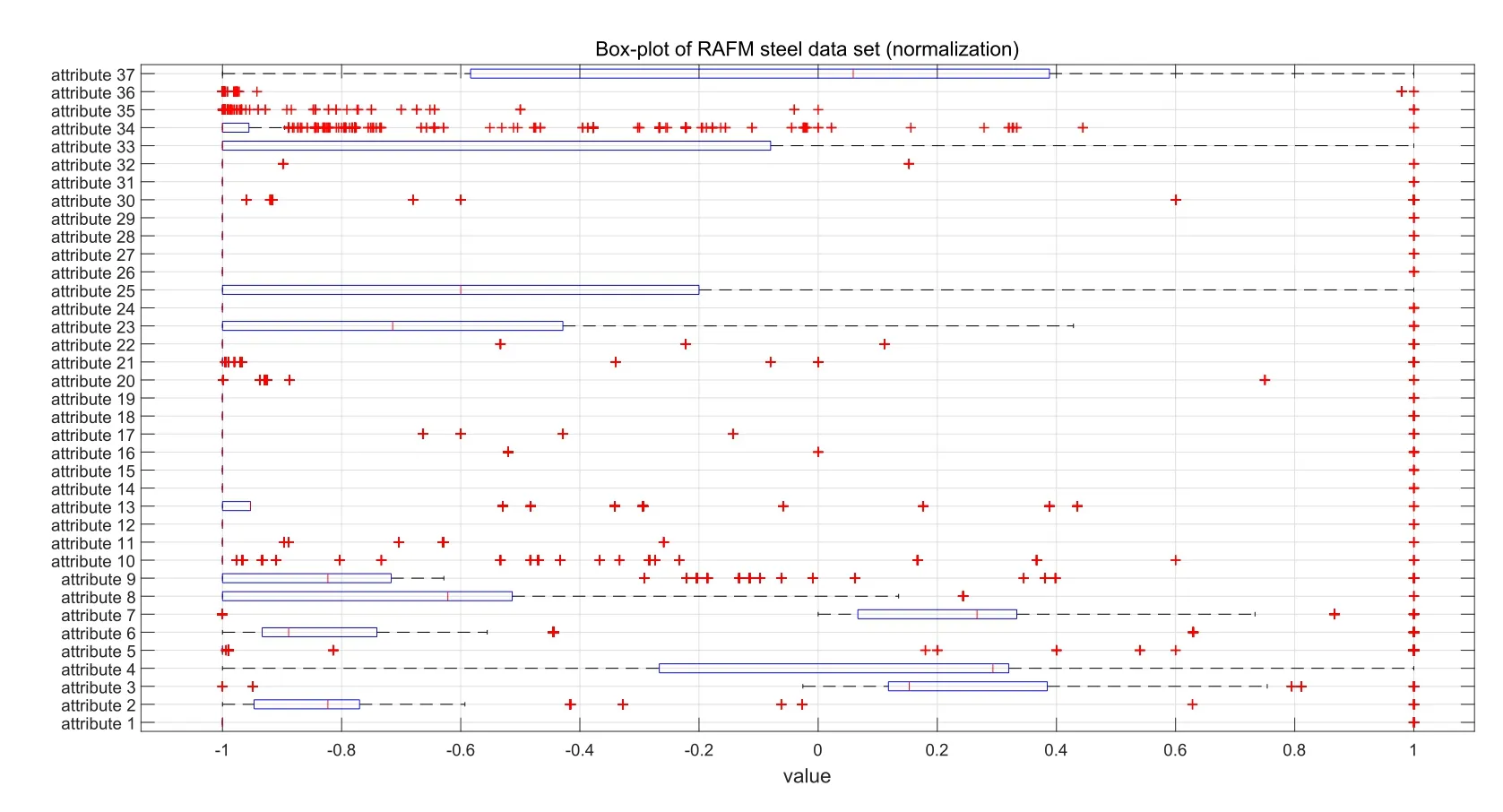
Figure2:The box-plot of 37 attribute values of RAFM steel shows that most of the attribute distributions are asymmetrical.In addition,there are many outliers

The distribution of data can affect the training process of the prediction model.Compared with the skewed distribution,the symmetry of the data contains a lot of information,and the distribution of information is more balanced,which will ease the learning task of the prediction model.In order to comprehensively analyze the data sets of RAFM steel,we use the box-plot in statistics to analyze it.It contains six data nodes,from which a set of data is arranged from large to small,respectively,to calculate the upper edge of the data,the upper four digits Q3,the median,the lower four digits Q1,the lower edge,and an exception value(outliers).The specific content of the box diagram can be referred to the work of Robert Mcgill et al.[Mcgill,Tukey and Larsen(1978)].Fig.2 shows the data symmetry and outliers by using box diagrams to display the original data.The graph shows that the set of attributes presents asymmetrical distribution,and there are many outliers(’+’representing outliers),which has a great challenge to the prediction results.Therefore,we must be able to find a model with strong anti noise ability,strong robustness and high generalization performance.It is difficult to use the traditional method,which will affect the final stability of the model.

3 SVR yield stress model of RAFM steel

Among a large number of heuristic search algorithms,different algorithms have different application scenarios. For example, the traditional genetic algorithm process is too complex for prediction of yield stress of RAFM steel[Zhang and Zhou(2016)],particle swarm optimization(PSO)algorithm is not good for solving discrete processing problem,it is easy to fall into the local optimum[Du(2016);Zhu and Cai(2016)].Simulated annealing algorithm has many advantages,such as fast convergence speed and efficient algorithm.So,it is often applied to various optimization methods[Chen,Zou and Wang(2016)].Based on these advantages,this study uses simulated annealing algorithm as the main optimization tool.This section will introduce the improved annealing method and the model of yield stress based on the SVR yield stress model of RAFM steel.Most search algorithms adopt the heuristic search method,but the ability to use information is deficient.Therefore,it is essential to improve the traditional annealing search algorithm by combining search information.

3.1 GDM-SA search algorithm

To accurately adjust the parameters of the SVR model,the simulated annealing algorithm must be improved to obtain the simulated annealing algorithm based on a smooth convex optimization and the gradient descent search algorithm,known as the GDM-SA algorithm.Compared with the traditional search algorithm,the GDM-SA algorithm can be used as a global search,and the algorithm can address the problem that the exact algorithm cannot be solved when the scale of the data is large.In the traditional simulated annealing algorithm,the general process is as follows.

1.Initialization:Set a high enough initial temperatureT0,and make T=T0,random initialization solutionS1,markov chain length L.

2.A new solutionS2is generated from the currentS1random perturbation.

3.Calculating the increment ofS2Δf=f(S1)-f(S2).

4.IfΔf＜0,accept the current solution,otherwise the new solution can only be accepted by the probability of exp(-Δf/T).

5.If the iterative condition is satisfied,save the optimal solution as is and end the program.Otherwise,perform do cooling according to the decay function and return to Step(2).

In the process of cooling,it is difficult to determine when the cooling achieves stable status.The traditional method is to fix the length of a markov chain directly.The problem is highly complex in that the objective functions in reality are always complex functions with multiple stagnation points,multiple saddle points,non-smoothness and other characteristics,and there are multiple local minima.Therefore,ordinary optimization methods will face more severe challenges.This paper uses a gradient descent algorithm to improve the range of the search region in the process of cooling.At the same time,this paper uses gradient data to give the algorithm local directivity.

In the process of annealing,if the number of iterations times is k,try to find the solution that meets the accuracy requirement in the K iterations.The algorithm tends to be stable at current temperature,and then proceed to the next iteration.

Given the following sets of training samples

(X1,Y1),(X2,Y2),(X3,Y3),...,(Xk,Yk)

The error calculation formula used in the K iteration:

After K times iteration,define the measure of overall cumulative error

Satisfying

In fact,

The above statements shall satisfy the independence assumption.Certainly,it is impossible to be completely independent in practice because there are overlapped parts of data samples on the training set,and there will be correlations between the trained learners depending on the actual situation.

The error in the K iteration isEk,∀Ek∈[τk,ηk],∀є-→0,according to the Hoeffding inequality,it has

The above shows that the precision of system itself has an exponential increase after K times[Ruxton(2010)],where K is a given number.

Considering that the mathematical properties of the cost functionEkare not good,use the exponential loss function as an alternative function.Some researchers already proved the consistency of the exponential loss function and the square loss function[Zhang(2004)].Thus,use the exponential loss function as the optimization objective,and the original formula becomes

Where g(k)=EkandEk～χis the mathematical expectation of the characteristic spaceχ.Then,use the method of smoothing convex optimization approach to optimize the new target function[Bubeck and bastien(2015)],that is to minimize the new objective functionι(k)

where theχis the characteristic space of the training sample set,and theψis the characteristic space of the overall sample set.

There are many ways such as the Lagrangian multiplier method to optimize the objective function,coordinate the descent method,the Newton method,the gradient descent method,and the variant methods derived from them.Using different optimization methods will have different effects on search results.The cost function has been converted to the exponential loss function [Singh,Singh,Singh et al.(2008)],therefore,use the gradient descent method to do optimization since the exponential loss function has good mathematical properties.

The gradient descent method requires that the following sequence can be constructed:

And requiring

In this instance,we used the idea of relaxation and approximation,and constructed a series of relaxation variables to approach the real functions.With the increase in the iteration times,and the contracted sequences,we can finally guarantee algorithm convergence.In practice,µis a step factor.To ensure convergence quickly,the direction of the descent should be in the negative direction of the gradient.The next section will deduce the optimization problem for this study.

During the iterative process,given that the error of theitime isEi,perform the second order Taylor expansion here because when the error is very small,the higher term of the Taylor expansion is the high order infinitesimal about the step factorµwhich is also called the learning rate in a neural network.The objective function can be approximately replaced by the following quadratic polynomial.

The upper form is the approximation function that is formed by the quadratic expansion structure.For the optimization functionι(k),here further are:

Mark∇is a gradient operator,andH[f(x)]is the second order Hessian matrix of thef(x)function[Powell(1979)].For the definition of the Hessian matrix,please refer to convex optimization theory[Bubeck(2014)],and the corresponding Hessian matrix here is:

In actual operation,because the calculation of the Hessian matrix absorbs extensive computing resources[Mcgill,Tukey and Larsen(1978)],the complexity grows exponentially with the increase of scale of the problem.Therefore,the relatively simple matrix(1/µ)Ithat is like the Hessian matrix is used to approximate the substitution andIis thekidentity matrix.From that,the new simplified formula is as follows:

The gradient vector operator near pointki+1is obtained by the quadratic approximation method.

Refer to convex optimization theory for the second order gradient analysis of the real variable function[Mcgill,Tukey and Larsen(1978)].The necessary condition for the existence of a first-order extreme point is to meet the requirement that the gradient is 0,using the following formula:

The upper form is the updated iteration formula of this algorithm.If the search ability cannot meet the specific data requirements,we can also use the second order gradient that is the information of the Hessian matrix to find a faster descent direction.The optimized objective function is as follows:

With reference to convex optimization theory,the necessary and sufficient conditions for the second order gradient analysis of a real variable function shows that in order to obtain the local optimal point of the original function(it is the minimum here),the first order gradient of the iterative increment is 0 and the second order gradient is positive.The Hessian matrix is required to be a positive de finite matrix.Therefore,it is necessary to find the constraint conditions.

The concept of a convex set,that is,for a given setSthat is a convex set,two arbitrary pointsAandBbelong toSand the line segments connecting them are also in the setS.It is as follows:

For the objective function,there is:

The objective functionιis a lower convex function.Therefore,any convex function satisfies the Jensen inequality

whenµ＞0,ιis a strong convex function.Therefore,the sufficient and necessary condition for the strong convex functionιto be an objective function that is defined onRis that if and only ifιCan be a quadratic differential and the Hessian matrix is a positive definite matrix.

From the above analysis, the objective function ι satisfies the constraints of the second order convex optimization.After the above constraints are satisfied,the second order algorithm of the smooth convex optimization can be used to analyze the second order gradient of the objective functionι.Therefore,it has the following:

Thus,the second order iterative formula for this study is obtained.

The upper form is called the Newton method,which uses the information of the second order gradient to optimize.The updated direction is more accurate,but the drawback is the inverse calculation of the Hessian matrix and the iterative process will also take up extensive of calculation resources.It is necessary to consider the actual situation for screening and this study gives two optimization methods above.

Applied to the cooling process during annealing,searching the optimal value in the process of cooling under the current temperature by the above algorithm,the algorithm will converge to an optical point and end the search.The algorithm will reach the stable status of the cooling process and start the next round of temperature cooling.The pseudo code of the whole process is represented in reference Tab.2.

Tab.2 is the use of pseudo code to explain the main program of the combinative annealing algorithm.The traditional annealing algorithm will set a fixed metropolis inner loop chain,except the Steps 5～16,as a short-term equilibrium constraint condition at the current temperature.This balance is called a steady state under the current temperature.However,this approach is relatively fixed,and it is difficult to know whether it reached the steady state or not after the iteration.Therefore,the GDM algorithm is designed to automatically adjust and optimize the algorithm to reach balance by the given precision value.Compared with traditional SA algorithms,the GDM algorithm is more flexible and the scope of the search space is also expended.

Table2:Improved simulated annealing GDM-SA algorithm

3.2 Comparison with unimproved algorithms

Compared with unimproved annealing algorithms,the simulated annealing algorithm of GDM has the advantages of a wider search range and easing of the premature local optimization.To verify the above advantages,chose the following complex functions as the test target to search the minimum of functionf(x1,x2).The function formula is

This function has numerous local minimum points,and it is easy to find that the global minimum of this function isx1=0,x2=0.At this point,f(x)takes the global minimum value of 1,that is

After selecting certain tasks,perform the comparison and analysis of the search capability between the simulated annealing algorithm improved by the GDM algorithm and the previous one.Set the same annealing parameters.The attenuation parameter is 0.95.The step factor is 10(force to control the disturbance).The initial temperature is 100,and the tolerance is 0.0001.The learning rate of GDM is 0.001.The maximum number of iterations is 4000.The minimum change curve of functionf(x)obtained in the iterative process is calculated as shown in Fig.3 below.

Fig.3 shows the results of calculating the minimum value of the given complex function on the examples given in this study.Under the same conditions,we compare the traditional simulated annealing algorithm,GDM-SA algorithm,particle swarm optimization algorithm and artificial bee colony(ABC)algorithm[Gao,Suganthan and Pan(2016)].The average results of each algorithm are obtained by running several times,and then the graph of search results changing with the number of iterations is drawn.It can be seen that the traditional optimization algorithm falls into the local optimum after the search,such as the traditional simulated annealing algorithm with an optimum value of 1.775,particle swarm optimization with an optimum value of 1.996,artificial bee colony with an optimum value of 2.063.The optimal value of GDM-SA algorithm is 1.498,and the search space is wide.Our explanation is that in the process of searching,we can make full use of the advantages of accurate search to find the best value after falling into the local optimal value,and at the same time,we can jump out of the local optimal value by combining the idea of annealing algorithm.Finally,our improved algorithm obtains better results than a single heuristic algorithm.However,the improved annealing algorithm of GDM can almost achieve a global optimal solution.Therefore,Fig.3 shows that the improved simulated annealing algorithm has a stronger searching ability,faster convergence speed and wider search scope.The above experiment is only a method to compare under the same conditions.When the temperature rises appropriately,the traditional simulated annealing algorithm can also approach the global minimum.

Figure3:The search results of GDM-SA algorithm and traditional simulated annealing algorithm,particle swarm optimization algorithm and artificial bee colony algorithm on function extremum optimization problem.Each algorithm performs at least three experiments,and then the search results are averaged to plot the optimal value and the number of iterations.

The results above show that the SA algorithm combined with the GDM algorithm,known as the GDM-SA algorithm,has a strong search ability.Next,the parameters of SVR are optimized by the GDM-SA algorithm to get the spatial grid research results within the interval range of optimal value.This paper introduces the SVR model of GDM-SA below and later establishes the yield stress prediction model of SVR.

3.3 GDM-SA-SVR yield stress model

This study use the SVR model to establish the yield stress model[Huang and Tsai(2009)].The principle of the SVR model is referred to the work of Vapnik[Cortes and Vapnik(1995)].

Referring to the data distribution of RAFM steel in Appendix A,the magnitude difference between different attributes is large.For example,carbon element content and the test temperature have 10000 orders of magnitude difference.In scientific calculation,it is necessary to prevent two very large numbers from calculating directly,which will lead to the loss of calculation precision and data information.Therefore,the normalization process is needed[Wang and Tang(2015)].The minimum and maximum normalized normalization formula is used here.

The strategy used in this paper is using the improved simulated annealing algorithm GDM-SA to optimize the penalty factor C of SVR and the kernel function parameter G(gamma)to get an approximate interval of extreme value.Meanwhile,for the regression error threshold parameterepsilon(general experience valueis 0.1),when the error is less than the modified value,it will not be punished,and the value will be punished when the error is bigger than the modified value.That is equivalent to the expected regression precision,so it has a significant effect on the result.In order to obtain more accurate results,we set a more subtle adjustment interval.Then,use the space grid search algorithm for accurate search[Liu,Liu and Yang(2006)].The combination of rough and precise search can effectively approximate the global optimal solution.

Train the model on a training set by the annealing algorithm[Ginneken and Van(2016)].Calculate the mean square error.The formula used in the K iteration is the mean square error formulaEk,above.(Refer to the definition in the last chapter).

Combine with the above design model to design a preliminary algorithm to iterate and optimize parametersCandGof SVR.To obtain more solutions,a more robust method is used to save the number ofmoptimal solutions after each iteration.Next,the number ofMoptimal solutions is sorted by the merging sort and stored in the matrix structure and the final product is output.To date,the annealing algorithm SA was improved by the GDM algorithm to optimize the SVR model,and saved the number of m best optimal solutions of the SVR model.The whole flow chart is shown as the Fig.4.The related attenuation parameters are set to 0.95,the step factor is 10(force to control disturbance),the initial temperature is 80,the tolerance is 0.0001,the GDM learning rate is 0.001,the maximum iteration number is 2000. Tab. 3 shows that 10 optimal values were selected after an iteratedannealing algorithm.

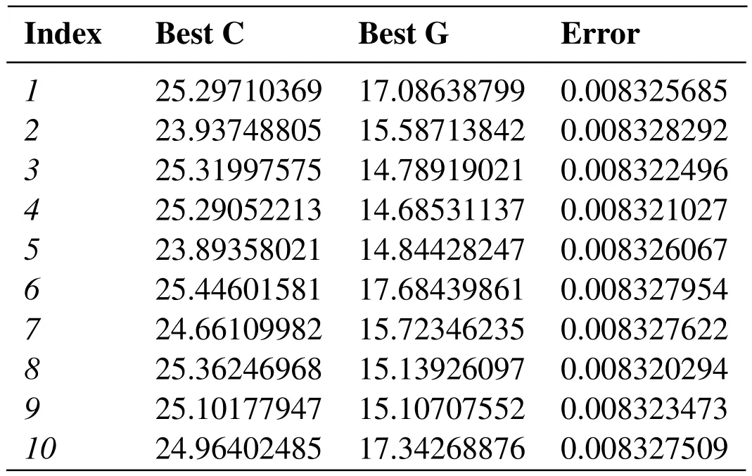
Table3:The best parameter values from different groups in a certain iteration(here epsilon =0 . 1)

Excessive penalty parameters will increase the accuracy of the training set but will lead to overfitting.In practice,we are inclined to choose relatively small parameter values.After many times of simulated annealing algorithm optimization,the final optimal value isC=16,G=8 andepsilon=0.0065.After initial determination of the optimal range,start the space grid search [Liu,Liu and Yang (2006)].

Figure4:Flowchart of improved simulated annealing algorithm.The improved algorithm process is more complex,and search ability is enhanced

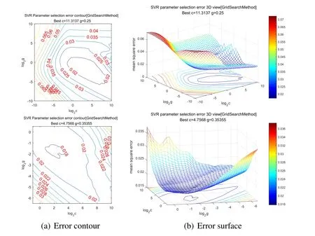
Figure5:Error contour and surface map after multiple iterations.Every iteration,the search area will be further reduced,and we can then determine the global optimal solution through repeated iterations

Take the sampling points of two dimensions in the optimal value interval calculated by the annealing algorithm,which is the test point of the parametersCandG.Taking the mean square error as the evaluation standard,make the three-dimensional coordinate diagram of the error of parametersCandGand draw the corresponding isogram.By analyzing the contour lines,the search range is further reduced and is repeatedly iterative to obtain the parameters that meet the requirements of the error precision and finally end the algorithm.After repeated iteration through the above methods,the parametersCandGwith small errors are finally approximated,and the value is assigned to the SVR model to retrain the model on the training set and finally obtain a relatively ideal model.Through the preceding analysis,for the extremum optimization problem of complex functions,find the optimal value by a heuristic algorithm (most are locally optimal) and then,after repeatedly iterative analysis,it can approach the global optimum infinitely [Zien,Kramer and Sonnenburg(2009)].

To date,an SVR model of 37 attribute variables on yield strength YS has been established.The following is the test and prediction analysis of the mode.

4 Test and analysis of the model

4.1 Model learning

When evaluating the performance of a model,a very important index is the learning situation of the training samples.Lack of learning will lead to underfitting,and the prediction results will reflect the high deviation characteristics.Overlearning will learn some features of the sample itself(for example,sample noise),and there will be overfitting at this time.The prediction results have a high variance characteristic.The ideal situation is to make a compromise between underfitting and overfitting.The generalization performance of the model is the best at this time.Overfitting and underfitting always accompanied the whole process of machine learning.Many factors are needed to be considered in the training model,and another important reason is that there is not a complete theory to guide a model for meeting the main problems in the process of establishing the model,such as training guidance and evaluating sample information.Even so,there still are some computational learning theories that can be used to analyze the learning model.

For a training set,we assume that learning satisfies the requirement by reaching a certain precision,є[Zeugmann(2016)],and it is recorded as timeh,the number of samples ist,and in the iterative training process,define the hypothesis space R.Next comes

when the number of samplestis big,the empirical error ofHCan be approximated to replace the generalization error.Given the hypothetical space R,whent→∞,the right side of the inequality is 0.There must be a hypothesis that the generalization error is minimal to guarantee the learning process.The following Fig.6 shows the learning of the sample after the final model training.

The training set used in this paper selects 1711 data training models from a random disorder sequence,and the remaining 100 data training models are used to verify the model.In the process of training the model,Fig.6(a)is over fitting learning the situation.Fig.6(b)is the learning situation between under fitting and over fitting,that is,learning the characteristics of samples,and noisy data not learned here,so there are some large deviations.This phenomenon is a normal.The data itself not only contains the noise data points but also the contradictory data points.

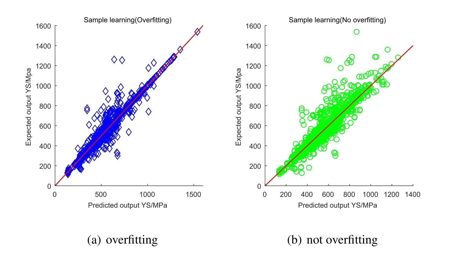
Figure6:Overfitting and not overfitting sample learning

4.2 Model comparison

To verify the performance of the model,compare the model with other similar models including ANN,random forest,linear regression and general regression neural network(GRNN).Train these models on the same set of data and then test these models on the same test set.Get the absolute error (residual) and error distribution of the predicted results.Perform test results statistics with the similar models.Fig.7 to Fig.11 is the result of error analysis.

The Tab.4 is a specific statistical analysis table.In the filed of ma ch inelearning,use statistical methods to test regression problems.and then,we obtain the residuals of prediction results and expected results on test sets.Perform statistical analysis of residual data by the commonly statistics including mean,maximum deviation,variance,standard deviation and mean square error (MSE) and goodness of fit (also called coefficient of determination).In general,the mean value of error obeys a normal distribution,and the closer to 0,the better the mean value of error is.The smaller the value of the maximum deviation,variance,standard deviation and mean square error are,the better the parameters themselves are.When the goodness of fit,known as the coefficient of determinationR2,is the closer to 1,the better the effect of the regression is.Tab.4 is the BP neural network,random forest,linear regression,generalized regression neural network and the GDM-SA-SVR algorithm used in this paper.It is obvious that GDM-SA-SVR has much better performance than other similar algorithm models in addition to the relevant smaller disadvantages.Therefore,the GDM-SA-SVR algorithm model is effective.

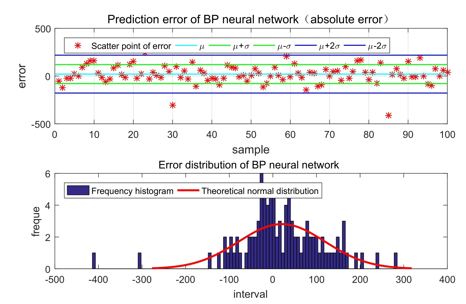
Figure7:Absolute error and frequency distribution histogram of BP neural network

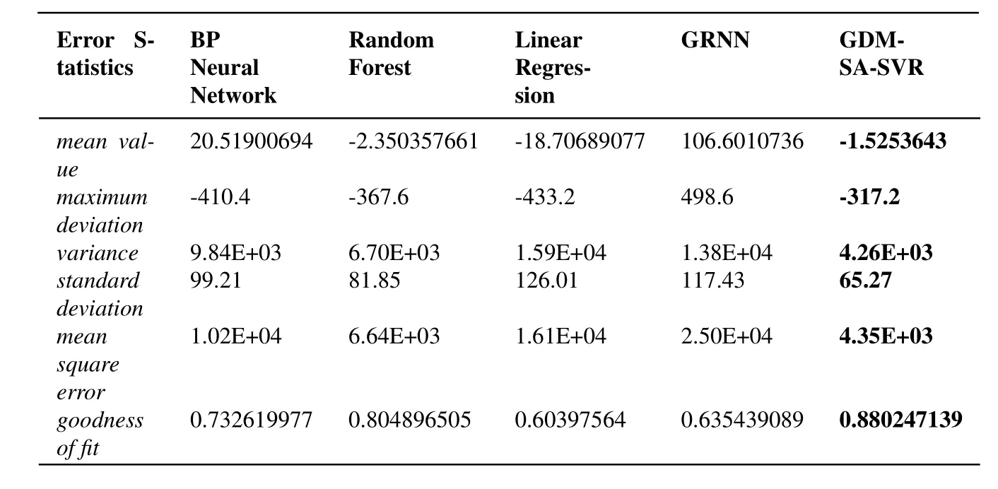
Table4:Performance comparison of BP neural network,random forest,linear regression,GRNN(generalized regression neural network)and GDM-SA-SVR algorithm on test set

Figure8:Absolute error and frequency distribution histogram of random forest

4.3 Significance test of the regression effect

The content of the previous section has explored the learning situation of the model for sample data and only assesses the ability of a model to store characteristic information of a data sample.Since the partition of a training set is completely independent,the performance of a test set is truly to show the predictability of the model when the model is used to predict.Given a test set that is not trained,the prediction effect of the model is different from the reality.

Fig.12 shows that 96 of the 100 data points on the test set fall within the two times sigma range of the prediction curve,and only four of the number are out of the range.The regression effect is very obvious from preliminary judgment,but for further analysis,it is necessary to test the results and the actual results by theT-test[Ruxton(2010)],it is uses thetdistribution theory to deduce the probability of occurrence of differences,so as to compare whether the difference between the two averages is significant.Therefore,it is possible to test whether there is a significant difference between the predicted result and the actual result.

For the original problem,it is assumed that there is a linear relationship between the predicted results and the actual results,and the regression coefficient set asb.

1.Putting forward the original hypothesis of regression coefficient

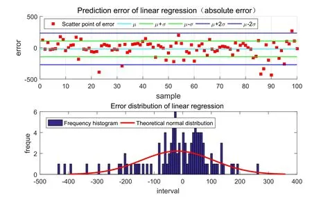
Figure9:Absolute error and frequency distribution histogram of linear regression

2.Structural statistics T,and satisfy

3.Given the significance levelα(0＜α＜1)making

4.Get a rejection region

Calculate T statistics through the experimental results and the test results.Accept the original hypothesis if the rejection region is not satisfied,that means the predicted effect does not have a linear relationship.Otherwise,the prediction effect has a linear relationship.The effect of regression is remarkable.

For a given confidence levelα=0.01,calculate the results T1=35.7328.There are 100 data points in the test set.When the degree of freedom is greater than 45,the T statistic is approximates the standard normal distribution,where T≈Z.Therefore,in theα=0.01 confidence level,check the table to get Z=2.57,that is,T1＞T.Therefore,reject the original hypothesis,and there is 99%confidence that the predictive value and the actual value of the regression effect is obvious.

Figure10:Absolute error and frequency distribution histogram of GRNN

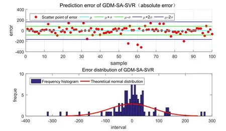
Figure11:Absolute error and frequency distribution histogram of GDM-SA-SVR

Figure12:The predictive effect of the GDM-SA-SVR model on the test set.From the graph,we can see that in the 100 training sets,(assuming that the error obeys normal distribution),only 4 points fall outside the prediction interval of 2 σ

In addition,there is another method (the correlation coefficient method used previously)that can test the effect of regression.This article does not make a detailed introduction about the correlation coefficient method and only gives the final result.Through calculation,the correlation coefficient fluctuates within the range of more than 0.8.At that point,the quantitative model set by statistical analysis evaluates that the SVR model has a significant regression effect on the test set.

5 Results and discussion

5.1 Prediction of test temperature

The test set data (100 pieces) is remarked before and after irradiation,and a scatter plot is drawn.The data are influenced by the mutual influence of different attributes.Therefore,the data have a certain dispersion,but the overall trend is more obvious.Extrapolation prediction is carried out within the extrapolated range of [100,1000] and a test temperature(K)[Aktaa and Schmitt (2006)].Use the trained SVR model to make the prediction curves of Fig.13 with the constraints before and after irradiation.Compared with the true scatter point data of the test set,the prediction curve has a better prediction effect.

The model prediction shows that in the temperature range of 100 K to 1000 K,when the temperature increases,the yield stress decreases as the curve in the Fig.13.The contrast of before irradiating and after irradiating indicates that doing the experiment in the test temperature range,within a given dose (the different effects from different doses,the size of irradiation dose in the curve diagram is approximately 0.024 dpa),the yield strength difference will decrease before and after irradiation[Wang,Zhang and Zhao(2017)].Since the sample of the training set includes a variety of alloy materials,the prediction of the RAFM steel alloy material is in line with the test set.

Figure13:The predictive effect of the GDM-SA-SVR model on the test set.The trained model is given 0 or a number of irradiation parameters,and then the prediction curve is compared with the original data points.The original data points are distributed near the prediction curve.The GDM-SA-SVR algorithm has a good prediction effect

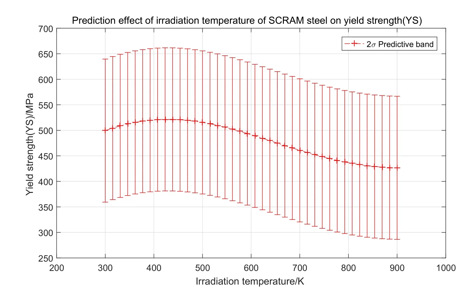
Figure14:Prediction interval of SCRAM steel in 2 σ ,where σ is the variance of the normal distribution of error

5.2 Prediction of radiation temperature

Below is the introduction of the reduced activation ferritic martensitic steel SCRAM steel,which was developed by a university with vacuum induction electric furnace smelting and argon protective atmosphere electroslag re-melting technology.The main chemical components are shown in Tab.5.

For the above SCRAM steel,give the same test temperature and irradiation dose to investigate the effect of different irradiation temperatures on the yield strength(YS)of SCRAM steel.

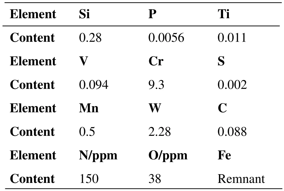
Table5:Chemical composition of SCRAM steel(wt%)

Fig.14 is the prediction interval of SCRAM steel in 2σ.In the irradiation temperature range [300,900] (unit K),the yield strength variation interval slowly increases first in the range of [200,800],and then decreases (MPa).Most of the radiation temperature range of the training set is arranged in 273 K to 900 K,so the prediction of extrapolation to SCRAM steel has a certain reliability.More accurate analysis needs to be compared with real experimental data.

Figure15:The prediction line of radiation temperature of SCRAM steel at different doses.The radiation dose was 0.05,0.18,1.3,10.1,22.3,43.3 and 88.6,respectively,and the corresponding prediction curve was calculated by GDM-SA-SVR model

Figure16:When the element composition of RAFM steel is changed,the prediction curves of different types of steels under different radiation doses are given

Fig.15 is the change of the yield strength of radiation at several doses in 0.05,0.18,1.3,10.1,22.3,43.3,and 88.6 (dpa) [Gaganidze and Aktaa (2013)].The prediction curve of the irradiation temperature in the range of [300,900] shows that the mutual influence of the physical mechanism of the two attributes is very complex,and in the studied dose range and a given range of irradiation temperature,the effect of the yield strength is not monotonic as there are many maximum or minimum values.If the physical background test is verified,the test points can be selected at the intersection point given by the forecast line.

The different irradiation doses have different effects on the yield strength.For example,the yield strength of the zirconium alloy will increase under irradiation,but the ductility will decrease [Lucon (2002)].This paper presents a research method to study the effects of different materials.First,the irradiation dose is evenly divided in a certain range,and then the SVR yield stress model is used to make the corresponding curve,so it can further study the effect of irradiation dose on the different results.This method can be evaluated and contrasted in reference to the study of yield stress [Virgil’Ev,Kalyagina and Makarchenko(1979)].

5.3 Prediction of temperature

The effect of different steels on the irradiation dose is also different.Fig.16 is the prediction curve made through the SVR prediction model under the conditions of extracting 6 types of RAFM steels with different chemical compositions from the test data set and a given dose in range of [0,80] (dpa).The prediction curves all are first increased and then decreased,and different chemical compositions have different effects.Most of the data used in this dataset are in the range of [0,50].Therefore,a comparative analysis should be performed with the future experimental points if the over-dose prediction is done.In practical engineering applications,generally,there are no standard experimental data points as a contrast indication,so the method needs to be studied in combination with other methods [Lucon (2002)].

5.4 Combination prediction of test temperature and irradiation dose

The previous analysis of the original data shows that there are multiple collinear dependencies among some attributes.To study the effect of this dependency on the model,a three-dimensional graph must be made to do visualization analysis of the SVR model.In Fig.17,350 K,436 K,600 K and 783 K are taken as irradiated temperature points corresponding to the combined influence of radiation dose and test temperature on the predicted surface.Clearly,the images of different irradiated surfaces have changed greatly.At the same time,it is worthy noticing that there are few data points in the boundary range,so the model will cause a deviation in the process of learning.

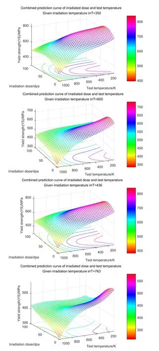
Figure17:The combined effect of test temperature and irradiation dose.The irradiation temperature is 350 K,436 K,600 K and 763 K,and the combined effect of the irradiation dose and the test temperature on yield strength is calculated by the GDM-SA-SVR model

6 Conclusions

In this paper,we use data mining technology,through statistical analysis of data distribution symmetry to further prepare for our screening model.Correlation can describe the collinearity of attributes and analyze the stability of the model.Next,we uses the technique of convex optimization theory to improve the traditional SA algorithm.Then,get the GDMSA algorithm is obtained with stronger search ability.After tests with complex optimal problems test,compared with the traditional SA algorithm under the same conditions,the GDM-SA algorithm has faster convergence speed,less falling into local optima and wider search ability.Therefore,use the improved simulated annealing algorithm (GDMSA) to optimize the parameters of the SVR model.Finally,a GDM-SA-SVR yield stress prediction model is derived for RAFM steel yield strength.

By comparison,the RAFM steel yield strength prediction model is better than ANN,linear regression,random forest and GRNN.In summary,it is concluded that the hybrid model composed of simulated annealing algorithm and support vector machine can achieve superior performance for compared with ANN,linear regression,GRNN,and random forest.The possible reason is that,from the distribution of the dataset,the data distribution is sparsely presented,which fits the prediction mechanism of the support vector machine.Because of data dispersity and sparsity,SVM can classify data better when it is mapped to the feature space.The soft interval is small,and the error is also small.Therefore,it is also very important to do data mining for original data,which is helpful for subsequent research.These results may help to guide the development direction of the model in the future as follows.

The SVR model uses a single kernel model while the best kernel function in the experiment is the Gauss kernel or the sigmoid kernel.Therefore,the use of multi-core models will achieve better results in facing of different data sets,which is also a heavily studied research field in SVR.In addition to the nature of the model itself,the data sets shall also be considered.If there are new data in the future,adding the new data into the data set to retrain the model can get better prediction ability than the current dataset,and the model is more accurate.

Acknowledgement:The research is supported by “National Natural Science Foundation of China” under Grant No.61572526,and thanks to Mr.He from the material radiation effect team of the China Institute of Atomic Energy.With the help and guidance of Mr.He and Mr.Deng,the experiment was successfully conducted,and the results were greatly improved,which enhanced the structure of this article.Thanks to the editor for giving detailed comments,the quality of the article can be improved.

Appendix A.Statistic information of sample data

Reference Tab.6.

Table6:Basic information of the input parameters