Nonlinear Bayesian Estimation:From Kalman Filtering to a Broader Horizon

Huazhen Fang,Ning Tian,Yebin Wang,Senior MengChu Zhou,and Mulugeta A.Haile

I.INTRODUCTION

AS a core subject of control systems theory,state estimation for nonlinear dynamic systems has been undergoing active research and development for a few decades.Considerable attention is gained from a wide community of researchers,thanks to its significant applications in signal processing,navigation and guidance,and econometrics,just to name a few.When stochastic systems,i.e.,systems subjected to the effects of noise,are considered,the Bayesian estimation approaches have evolved as a leading estimation tool enjoying significant popularity.Bayesian analysis traces back to the 1763 essay[1],published two years after the death of its author,Rev.Thomas Bayes.This seminal work was meant to tackle the following question:“Given the number of times in which an unknown event has happened and failed:Required the chance that the probability of its happening in a single trial lies somewhere between any two degrees of probability that can be named”.Bayes developed a solution to examine the case of only continuous probability,single parameter and a uniform prior,which is an early form of the Bayes’rule known to us nowadays.Despite its preciousness,this work remained obscure for many scientists and even mathematicians of that era.The change came when the French mathematician Pierre-Simon de Laplace rediscovered the result and presented the theorem in the complete and modern form.A historical account and comparison of Bayes’and Laplace’s work can be found in[2].From today’s perspective,the Bayes’theorem is a probability-based answer to a philosophical question:How should one update an existing belief when given new evidence[3]?Quantifying the degree of belief by probability,the theorem modifies the original belief by producing the probability conditioned on new evidence from the initial probability.This idea was applied in the past century from one field to another whenever the belief update question arose,driving numerous intriguing explorations.Among them,a topic of perennial interest is Bayesian state estimation,which is concerned with determining the unknown state variables of a dynamic system using the Bayesian theory.

The capacity of Bayesian analysis to provide a powerful framework for state estimation has been well recognized now.A representative method within the framework is the wellknown Kalman filter(KF),which“revolutionized the field of estimation...(and)opened up many new theoretical and practical possibilities”[4].KF was initially developed by using the least squares in the 1960 paper[5]but reinterpreted from a Bayesian perspective in[6],only four years after its invention.Further envisioned in[6]was that“the Bayesian approach offers a unified and intuitive viewpoint particularly adaptable to handling modern-day control problems”.This investigation and vision ushered a new statistical treatment of nonlinear estimation problems,laying a foundation for the prosperity of research on this subject.

In this article,we offer a systematic and bottom-to-up introduction to major Bayesian state estimators,with a particular emphasis on the KF family.We begin with outlining the essence of Bayesian thinking for state estimation problems,showing that its core is the model-based prediction and measurement-based update of the probabilistic belief of unknown state variables.A conceptual KF formulation can be made readily in the Bayesian setting,which tracks the mean and covariance of the states modeled as random vectors throughout the evolution of the system.Turning a conceptual KF into executable algorithms requires certain approximations to nonlinear systems;and depending on the approximation adopted,different KF methods are derived.We demonstrate three primary members of the KF family in this context:extended KF(EKF),unscented KF(UKF),and ensemble KF(EnKF),all of which have achieved proven success both theoretically and practically.A review of other important Bayesian estimators and estimation problems is also presented brie fl y in order to introduce the reader to the state of the art of this vibrant research area.

where xk∈Rnxis the unknown system state,and yk∈Rnythe output,with both nxand nybeing positive integers.The process noise wkand measurement noise vkare mutually independent,zero-mean white Gaussian sequences with covariances Qkand Rk,respectively.The nonlinear mappings f:Rnx→Rnxand h:Rnx→Rnyrepresent the process dynamics and the measurement model,respectively.The system in(1)is assumed input-free for simplicity of presentation,but the following results can be easily extended to an input-driven system.

The state vector xkcomprises a set of variables that fully describe the status or behavior of the system.It evolves through time as a result of the system dynamics.The process of states over time hence represents the system’s behavior.Because it is unrealistic to measure the complete state in most practical applications,state estimation is needed to infer xkfrom the output yk.More specifically,the significance of estimation comes from the crucial role it plays in the study of dynamic systems.First,one can monitor how a system behaves with state information and take the corresponding actions when any adjustment is necessary.This is particularly important to ensure the detection and handling of internal faults and anomalies at the earliest phase.Second,high-performance state estimation is the basis for the design and implementation of many control strategies.The past decades have witnessed the rapid growth of control theories,and most of them,including optimal control,model predictive control,sliding mode control and adaptive control,premise the design on the availability of state information.

While state estimation can be tackled in a variety of ways,the stochastic estimation has drawn remarkable attention and been profoundly developed in terms of both theory and applications.Today,it is still receiving continued interest and intense research effort.From a stochastic perspective,the system in(1)can be viewed as a generator of random

II.A BAYESIAN VIEW OF STATE ESTIMATION

We consider the following nonlinear discrete-time system:vectors xkand yk.The reasoning is as follows.Owing to the initial uncertainty or lack of knowledge of the initial condition,x0can be considered as a random vector subject to variation due to chance.Then,f(x0)represents a nonlinear transformation of x0,and its combination with w0modeled as another random vector generates a new random vector x1.Following this line,xkfor any k is a random vector,and the same idea applies to yk.In practice,one can obtain the sensor measurement of the output at each time k,which can be considered as a sample drawn from the distribution of the random vector yk.For simplicity of notation,we also denote the output measurement as ykand the measurement set at time k as Yk:={y1,y2,...,yk}.The state estimation then is to build an estimate of xkusing Ykat each time k.To this end,one’s interest then lies in how to capture p(xk|Yk),i.e.,the probability density function(PDF)of xkconditioned on Yk.This is because p(xk|Yk)captures the information of xkconveyed in Ykand can be leveraged to estimate xk.

A “prediction-update”procedure1The two steps are equivalently referred to as “time-update”and “measurement-update”,or “forecast”and “analysis”,in different literature.can be recursively executed to obtain p(xk|Yk).Standing at time k-1,we can predict what p(xk|Yk-1)is like using p(xk-1|Yk-1).When the new measurement ykconveying information about xkarrives,we can update p(xk|Yk-1)to p(xk|Yk).Characterizing a probabilistic belief about xkbefore and after the arrival of yk,p(xk|Yk-1)and p(xk|Yk)are referred to as thea priorianda posterioriPDF’s,respectively.Specifically,the prediction at time k-1,demonstrating the pass from p(xk-1|Yk-1)to p(xk|Yk-1),is given by

Let us explain how to obtain(2).By the Chapman-Kolmogorov equation,it can be seen that

which,according to the Bayes’rule,can be written as

It reduces to(2),because p(xk|xk-1,Yk-1)=p(xk|xk-1)as a result of the Markovian propagation of the state.Then on the arrival of yk,p(xk|Yk-1)can be updated to yield p(xk|Yk),which is governed by

The above equation is also owing to the use of the Bayes’rule

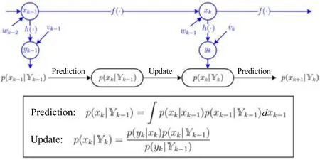
Fig.1.The Bayesian filtering principle.The running of a dynamic system propagates state xkthrough time and produces output measurement ykat time k.For the purpose of estimation,the Bayesian filtering principle tracks the PDF of xkgiven the measurement set Yk={y1,y2,...,yk}.It consists of two steps sequentially implemented:prediction from p(xk-1|Yk-1)to p(xk|Yk-1),and update from p(xk|Yk-1)to p(xk|Yk)upon the arrival of yk.

Note that we have p(yk|xk,Yk-1)=p(yk|xk)from the fact that ykonly depends on xk.Then,(3)is obtained.Together,(2)and(3)represent the fundamental principle of Bayesian state estimation for the system in(1),describing the sequential propagation of thea priorianda posterioriPDF’s.The former captures our belief over the unknown quantities in the presence of only the prior evidence,and the latter updates this belief using the Bayesian theory when new evidence becomes available.The two steps,prediction and update,are executed alternately over time,as illustrated in Fig.1.

Looking at the above Bayesian filtering principle,we can summarize three elements that constitute the thinking of Bayesian estimation.First,all the unknown quantities or uncertainties in a system,e.g.,state,are viewed from a probabilistic perspective.In other words,any unknown variable is regarded as a random one.Second,the output measurements of a system are samples drawn from a certain probability distribution dependent on the concerned variables.They provide data evidence for state estimation.Finally,the system model represents transformations that the unknown and random state variables undergo over time.Originating from the philosophical abstraction that anything unknown,in one’s mind,is subject to variations due to chance,the randomness-based representation enjoys universal applicability even when the unknown or uncertain quantities are not necessarily random in physical sense.In addition,it can easily translate into a convenient“engineering”way for estimation of the unknown variables,to be shown in the following discussions.

III.FROM BAYESIAN FILTERING TO KALMAN FILTERING

In the above discussion,we have shown the probabilistic nature of state estimation and presented the Bayesian filtering principle(2)and(3)as a solution framework.However,this does not mean that one can simply use(2)and(3)to track the conditional PDF of a random vector passing through nonlinear transformations,because the nonlinearity often makes it difficult or impossible to derive an exact or closed-form solution.This challenge turns against the development of executable state estimation algorithms,since a dynamic system’s state propagation and observation are based on the nonlinear functions of the random state vector xk,i.e.,f(xk)and h(xk).Yet for the sake of estimation,one only needs the statistics(mean and covariance)of xkconditioned on the measurements in most circumstances,rather than a full grasp of its conditional PDF.A straightforward and justifiable way is to use the mean as the estimate of xkand the covariance as the confidence(or equivalently,uncertainty)measure.Reducing the PDF tracking to the mean and covariance tracking can significantly mitigates the difficulty in the design of state estimators.To simplify the problem further,certain Gaussianity approximations can be made because of the mathematical tractability and statistical soundness of Gaussian distributions(for the reader’s convenience,several properties of the Gaussian distribution to be used next are summarized in Appendix).Proceeding in this direction,we can reach a formulation of the KF methodology,as shown below.

In order to predict xkat time k-1,we consider the minimum-variance unbiased estimation,which gives that the best estimate of xkgiven Yk-1,denoted asˆxk|k-1,is E(xk|Yk-1)[7,Theorem 3.1].That is,

Inserting(2)into the above equation,we have

By assuming that wkis a white Gaussian noise independent of xk,we have xk|xk-1∼N(f(xk-1),Q)and then Rxkp(xk|xk-1)dxk=f(xk-1)according to Appendix(64).Hence,(5)becomes

With the use of(2)and Appendix(64),we can obtain

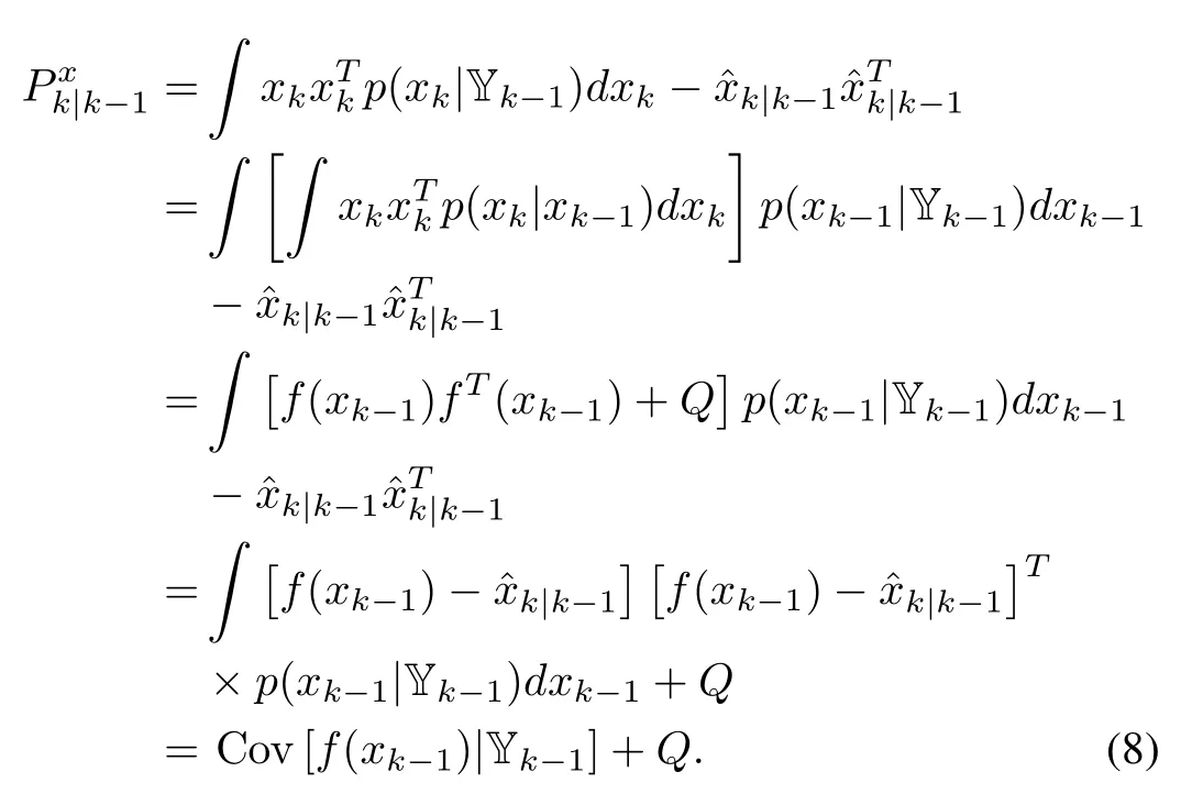
When ykbecomes available,we assume that p(xk,yk|Yk-1)can be approximated by a Gaussian distribution

The associated covariance is

It is noted that

Combining(10)and(11)with(12)yields

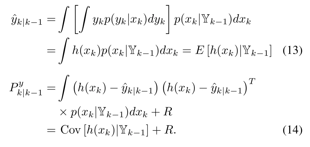
The cross-covariance between xkand ykis

For two jointly Gaussian random vectors,the conditional distribution of one given another is also Gaussian,which is summarized in(67)in Appendix.It then follows from(9)that a Gaussian approximation can be constructed for p(xk|Yk).Its mean and covariance can be expressed as

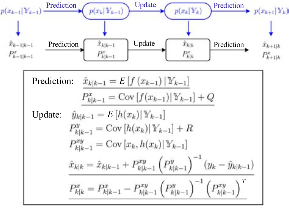
Fig.2. A schematic sketch of the KF technique.KF performs the prediction-update procedure recursively to track the mean and covariance of xkfor estimation.The equations show that its implementation depends on determining the mean and covariance of the random state vector through nonlinear functions f(·)and h(·).

Putting together(6)-(8),(13),(14)and(15)-(17),we can establish a conceptual description of the KF technique,which is outlined in Fig.2.Built in the Bayesian-Gaussian setting,it conducts state estimation through tracking the mean and covariance of a random state vector.It is noteworthy that one needs to develop explicit expressions to enable the use of the above KF equations.The key that bridges the gap is to find the mean and covariance of a random vector passing through nonlinear functions.For linear dynamic systems,the development is straightforward,because,in the considered context,the involved PDF’s are strictly Gaussian and the linear transformation of the Gaussian state variables can be readily handled.The result is the standard KF to be shown in the next section.However,complications arise in the case of nonlinear systems.This issue has drawn significant interest from researchers.A wide range of ideas and methodologies have been developed,leading to a family of nonlinear KFs.The three most representative among them are EKF,UKF,and EnKF to be introduced following the review of the linear KF.

IV.STANDARD LINEAR KALMAN FILTER

In this section,KF for linear systems is reviewed briefly to pave the way for discussion of nonlinear KFs.Consider a linear time-invariant discrete-time system of the form(

where:1){wk}and{vk}are zero-mean white Gaussian noise sequences with wk∼N(0,Q)and vk∼N(0,R),2)x0is Gaussian with x0∼N(x¯0,P0),and 3)x0,{wk}and{vk}are independent of each other.Note that,under these conditions,the Gaussian assumptions in Section III exactly hold for the linear system in(18).

The standard KF for the linear dynamic system in(18)can be readily derived from the conceptual KF summarized in Fig.2.Since the system is linear and under a Gaussian setting,p(xk-1|Yk-1)and p(xk|Yk-1)are strictly Gaussian according to the properties of Gaussian vectors.Specifically,xk-1|Yk-1∼N(xˆk-1|k-1,Pkx-1|k-1)and xk|Yk-1∼Here,one can letP0.According to(6)and(8),the prediction is

The update can be accomplished along the similar lines.Based on(13)-(15),we haveandThen,as indicated by(16)and(17),the updated state estimate is

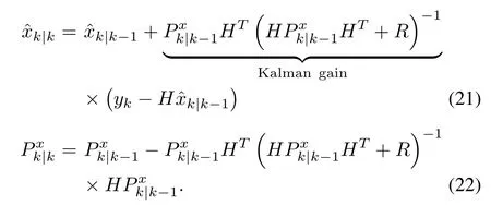
Together,(19)-(22)form the linear KF.Through the prediction-update procedure,it generates the state estimates and associated estimation error covariances recursively over time when the output measurement arrives.From a probabilistic perspective,andtogether determine the Gaussian distribution of xkconditioned on Yk.The covariance,quantifying how widely the random vector xkcan potentially spread out,can be interpreted as a measure of the confidence on or uncertainty of the estimate.A schematic diagram of the KF is shown in Fig.3(It can also be used to demonstrate EKF to be shown next).

Given that(F,H)is detectable andstabilizable,converges to a fixed point,which is the solution to a discrete-time algebraic Riccati equation(DARE)

This implies that KF can approach a steady state after a few time instants.With this idea,one can design a steady-state KF by solving DARE offline to obtain the Kalman gain and then apply it to run KF online,as detailed in[7].Obviating the need for computing the gain and covariance at every time instant,the steady-state KF,though suboptimal,presents higher computational efficiency than the standard KF.

V.REVIEW OF NONLINEAR KALMAN FILTERS

In this section,an introductory overview of the major nonlinear KF techniques is offered,including the celebrated EKF and UKF in the field of control systems and the EnKF popular in the data assimilation community.

A.Extended Kalman Filter

EKF is arguably the most celebrated nonlinear state estimation technique,with numerous applications across a variety of engineering areas and beyond[9].It is based on the linearization of nonlinear functions around the most recent state estimate.When the state estimatek-1|k-1is generated,consider the first-order Taylor expansion of f(xk-1)at this point:

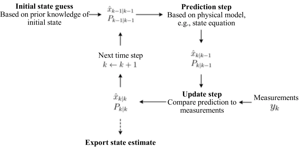
Fig.3.A schematic of the KF/EKF structure,modified from[8].KF/EKF comprises two steps sequentially executed through time,prediction and update.For prediction,xkis predicted by using the data up to time k-1.The forecast is denoted asand subject to uncertainty quantified by the prediction error covariance The update step occurs upon the arrival of new measurement yk.In this step,ykis leveraged to correctand produce the updated estimateMeanwhile,is updated to generateto quantify the uncertainty imposed on

For simplicity,let p(xk-1|Yk-1)be approximated by a distribution with meanand covarianceThen inserting(23)to(6)-(8),we can readily obtain the one-step forward prediction

Looking into(23),we find that the Taylor expansion approximates the nonlinear transformation of the random vector xkby an affine one.Proceeding on this approximation,we can easily estimate the mean and covariance of f(xk-1)once provided the mean and covariance information of xk-1conditioned on Yk-1.This,after being integrated with the effect of noise wkon the prediction error covariance,establishes a prediction of xk,as specified in(25)and(26).Afterk|k-1is produced,we can investigate the linearization of h(xk)around this new operating point in order to update the prediction.That is,

Similarly,we assume that p(xk|Yk-1)can be replaced by a distribution with meanand covarianceUs¡ing(27),the evaluation of(13)-(15)yields?Here,the approximate mean and covariance information ofand ykare obtained through the linearization of h(xk)aroundWith the aid of the Gaussianity assumption in(9),an updated estimate of xkis produced as follows:

Then,EKF consists of(25)and(26)for prediction and(29)and(30)for update.When comparing it with the standard KF in(19)-(22),we can find that they share significant resemblance in structure,except that EKF introduces the linearization procedure to accommodate the system nonlinearities.

Since the 1960s,EKF has gained wide use in the areas of aerospace,robotics,biomedical,mechanical,chemical,electrical and civil engineering,with great success in the real world witnessed.This is often ascribed to its relative easiness of design and execution.Another important reason is its good convergence from a theoretical viewpoint.In spite of the linearization-induced errors,EKF has provable asymptotic convergence under some conditions that can be satisfied by many practical systems[10]-[14].However,it also suffers from some shortcomings.The foremost one is the inadequacy of its first-order accuracy for highly nonlinear systems.In addition,the need for explicit derivative matrices not only renders EKF futile for discontinuous or other non-differentiable systems,but also pulls it away from convenient use in view of programming and debugging,especially when nonlinear functions of a complex structure are faced.This factor,together with the computational complexity at O(n3x),limits the application of EKF to only low-dimensional systems.

Some modified EKFs have been introduced for improved accuracy or efficiency.In this regard,a natural extension is through the second-order Taylor expansion,which leads to the second-order EKF with more accurate estimation[15]-[19].Another important variant,named iterated EKF(IEKF),iteratively re fines the state estimate around the current point at each time instant[18],[19].Though requiring an increased computational cost,it can achieve higher estimation accuracy even in the presence of severe nonlinearities in systems.

B.Unscented Kalman Filter

As the performance of EKF degrades for systems with strong nonlinearities,researchers have been seeking better ways to conduct nonlinear state estimation.In the 1990’s,UKF was invented[20],[21].Since then,it has been gaining considerable popularity among researchers and practitioners.This technique is based on the so-called“unscented transform(UT)”,which exploits the utility of deterministic sampling to track the mean and covariance information of a random variable passing through a nonlinear transformation[22]-[24].The basic idea is to approximately represent a random variable by a set of sample points(sigma points)chosen deterministically to completely capture the mean and covariance.Then,projecting the sigma points through the nonlinear function concerned,one obtains a new set of sigma points and then use them to form the mean and covariance of the transformed variable for estimation.

To explain how UT tracks the statistics of a nonlinearly transformed random variable,we consider a random variable x∈Rnand a nonlinear function z=g(x).It is assumed that the mean and covariance of x are¯x and Px,respectively.The UT proceeds as follows[22],[23].First,a set of sigma points{xi,i=0,1,...,2n}are chosen deterministically:

where[·]irepresents the ith column of the matrix and the matrix square root is defined byachievable through the Cholesky decomposition.The sigma points spread across the space around¯x.The width of spread is dependent on the covariance Pxand the scaling parameter λ,where λ =α2(n+ κ)-n.Typically,α is a small positive value(e.g.,10-3),and κ is usually set to 0 or 3-n[20].Then the sigma points are propagated through the nonlinear function g(·)to generate the sigma points for the transformed variable z,i.e.,

The mean and covariance of z are estimated as

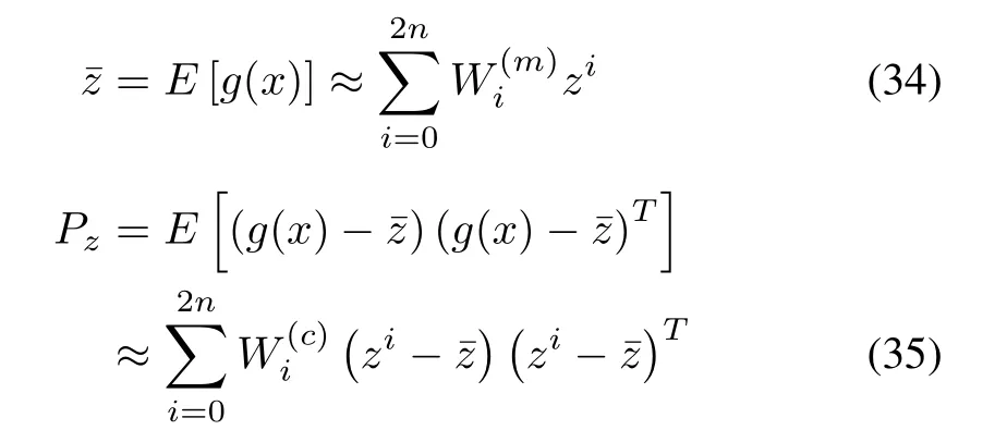
where the weights are

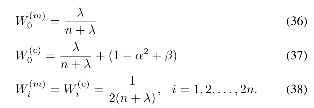
The parameter β in(37)can be used to include prior information on the distribution of x.When x is Gaussian,β=2 is optimal.The UT procedure is schematically shown in Fig.4.

To develop UKF,it is necessary to apply UT at both prediction and update steps,which involve nonlinear state transformations based on f and h,respectively.For prediction,suppose that the mean and covariance of xk-1,andare given.To begin with,the sigma points for xk-1are generated:

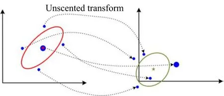
Fig.4. A schematic sketch of the UT procedure,adapted from[22].A set of sigma points(blue dots)are generated first according to the initial mean(red five-pointed star)and covariance(red ellipse)(left)and projected through the nonlinear function to generate a set of new sigma points(right).The new sigma points are then used to calculate the new mean(green star)and covariance(green ellipse).

Then,they are propagated forward through the nonlinear function f(·),that is,

These new sigma points are considered capable of capturing the mean and covariance of f(xk-1).Using them,the prediction of xkcan be achieved as follows:

By analogy,the sigma points for xkneed to be generated first in order to perform the update,which are

Propagating them through h(·),we can obtain the sigma points for h(xk),given by

The predicted mean and covariance of ykand the cross-covariance between xkand ykare as follows:

With the above quantities becoming available,the Gaussian update in(16)and(17)can be leveraged to enable the projection from the predicted estimatek|k-1to the updated estimate|k.

Summarizing the above equations leads to UKF sketched in Fig.5.Compared with EKF,UKF incurs a computational cost of the same order O()but offers second-order accuracy[22],implying an overall smaller estimation error.In addition,its operations are derivative-free,exempt from the burdensome calculation of the Jacobian matrices in EKF.This will not only bring convenience to practical implementation but also imply its applicability to discontinuous undifferentiable nonlinear transformations.Yet,it is noteworthy that,with a complexity of O()and operations of 2nx+1 sigma points,UKF faces substantial computational expenses when the system is high-dimensional with a large nx,thus unsuitable for this kind of estimation problems.

Owing to its merits,UKF has seen a growing momentum of research since its advent.A large body of work is devoted to the development of modified versions.In this respect,square-root UKF(SR-UKF)directly propagates a square root matrix,which enjoys better numerical stability than squaring the propagated covariance matrices[25];iterative refinement of the state estimate can also be adopted to enhance UKF as in IEKF,leading to iterated UKF(IUKF).The performance of UKF can be improved by selecting the sigma points in different ways.While the standard UKF employs symmetrically distributed 2nx+1 sigma points,asymmetric point sets or sets with a larger number of points may bring better accuracy[26]-[29].Another interesting question is the determination of the optimal scaling parameter κ,which is investigated in[30].UKF can be generalized to the so-called sigma-point KF(SPKF),which refers to the class of filters that use deterministic sampling points to determine the mean and covariance of a random vector through nonlinear transformation[31],[32].Other SPKF techniques include the central-difference KF(CDKF)and Gauss-Hermite KF(GHKF),which perform sigma-point-based filtering and can also be interpreted from the perspective of Gaussian-quadrature-based filtering[33].GHKF is to be further discussed in Section VII.

C.Ensemble Kalman Filter

Fig.5. A schematic of UKF.Following the prediction-update procedure,UKF tracks the mean and covariance of state xkusing sigma points chosen deterministically.A state estimate is graphically denoted by a red five-pointed-star mean surrounded by a covariance ellipse,and the sigma points are colored in blue dots.

Since its early development in[34]-[36],the ensemble KF(EnKF)has established a strong presence in the field of state estimation for large-scale nonlinear systems.Its design is built on an integration of KF with the Monte Carlo method,which is a prominent statistical method concerning simulation-based approximation of probability distributions using samples directly drawn from certain distributions.Basically,it maintains an ensemble representing the conditional distribution of a random state vector given the measurement set.The state estimate is generated from the sample mean and covariance of the ensemble.In view of the sample-based approximation of probability distributions,EnKF shares similarity with UKF;however,the latter employs deterministic sampling while EnKF adopts non-deterministic sampling.

Suppose that there is an ensemble of samples,for i=1,2,...,Ns,drawn from p(xk-1|Yk-1)to approximately represent this PDF.Next,let an ensemble of samples,for i=1,2,...,Ns,be drawn independently and identically from Gaussian distribution N(0,Q)in order to account for the process noise wk-1.Thencan hence be projected to generatea prioriensemblethat represents p(xk|Yk-1)as follows:

The sample mean and covariance of this ensemble can be calculated as:

which form the prediction formulae.

The update step begins with the construction of the ensemble for p(yk|Yk-1)by means of

with the associated sample covariance

The cross-covariance between xkand ykgiven Yk-1is

Once it arrives,the latest measurement ykcan be applied to update each member ofa prioriensemble in the way de fined by(16),i.e.,

Thisa posterioriensemble{}can be regarded as an approximate representation of p(xk|Yk).Then,the updated estimation of the mean and covariance of xkcan be achieved through:

The above ensemble-based prediction and update are repeated recursively,forming EnKF.Note that the computation of estimation error covariance in(54)and(61)can be skipped if a user has no interest in learning about the estimation accuracy.This can cut down EnKF’s storage and computational cost.

Fig.6.A schematic of EnKF.EnKF maintains an ensemble of sample points for the state vector xk.It propagates and updates the ensemble to track the distribution of xk.The state estimation is conducted by calculating the sample mean(red five-pointed-star)and covariance(red ellipse)of the ensemble.

EnKF is illustrated schematically in Fig.6.It features direct operation on the ensembles as a Monte Carlo-based extension of KF.Essentially,it represents the PDF of a state vector by using an ensemble of samples,propagates the ensemble members and makes estimation by computing the mean and covariance of the ensemble at each time instant.Its complexity is O(+Ns+ny+nx)(nx≫nyand nx≫Nsfor high-dimensional systems)[37],which contrasts with O(of EKF and UKF.This,along with the derivative-free computation and freedom from covariance matrix propagation,makes EnKF computationally efficient and appealing to be the method of choice for high-dimensional nonlinear systems.An additional contributing factor in this respect is that the ensemble-based computational structure places it in an advantageous position for parallel implementation[38].It has been reported that convergence of EnKF can be fast even with a reasonably small ensemble size[39],[40].In particular,its convergence to KF in the limit for large ensemble size and Gaussian state probability distributions is proven in[40].

VI.APPLICATION TO SPEED-SENSORLESS INDUCTION MOTORS

This section presents a case study of applying EKF,UKF and EnKF to state estimation for speed-sensorless induction motors.Induction motors are used as an enabling component for numerous industrial systems,e.g.,manufacturing machines,belt conveyors,cranes,lifts,compressors,trolleys,electric vehicles,pumps,and fans[41].In an induction motor,electromagnetic induction from the magnetic field of the stator winding is used to generate the electric current that drives the rotor to produce torque.This dynamic process must be delicately controlled to ensure accurate and responsive operations.Hence,control design for this application was researched extensively during the past decades,e.g.,[41]-[43].Recent years have seen a growing interest in speed-sensorless induction motors,which have no sensors to measure the rotor speed to reduce cost and increase reliability.However,the absence of the rotor speed makes control design more challenging.To address this challenge,state estimation is exploited to recover the speed and other unknown variables.It is also noted that an induction motor as a multivariable and highly nonlinear system makes a valuable benchmark for evaluating different state estimation approaches[43],[44].

The induction motor model in a stationary two-phase reference frame can be written as

where(ψdr,ψqr)is the rotor fl uxes,(ids,iqs)is the stator currents,and(uds,uqs)is the stator voltages,all de fined in a stationary d-q frame.In addition,ω is the rotor speed to be estimated,J is the rotor inertia,TLis the load torque,and y is the output vector composed of the stator currents.The rest symbols are parameters,where σ=Ls(1-/LsLr),α =Rr/Lr,β =Lm/(σLr),γ =Rs/σ + αβLm,µ=3Lm/(2Lr);(RsLs)and(Rr,Lr)are the resistance-inductance pairs of the stator and rotor,respectively;Lmis the mutual inductance.As shown above,the state vector x comprises ids,iqs,ψdr,ψqr,and ω.The parameter setting follows[45].Note that,because of the focus on state estimation,an open-loop control scheme is considered with uds(t)=380sin(100πt)and uqs(t)=-380sin(200πt).The state estimation problem is then to estimate the entire state vector through time using the measurement data of ids,iqs,udsand uqs.

In the simulation,the model is initialized with x0=[0 0 0 0 0]T.The initial state guess for all the filters is set to be0|0=[1 1 1 1 1]Tand=10-2I.For EnKF,its estimation accuracy depends on the ensemble size.Thus,different sizes are implemented to examine this effect,with Ns=40,100,200 and 400.To make a fair evaluation,EKF,UKF and EnKF with each Nsare run for 100 times as a means to reduce the influence of randomly generated noise.The estimation error for each run is defined asPk‖xk-k|k‖2;the errors from the 100 runs are averaged to give the final estimation error for comparison.

Fig.7 shows the estimation errors for ω along with ±3σ bounds in a simulation run of EKF,UKF and EnKF with ensemble size of 100(here,σ stands for the standard deviation associated with the estimate of ω,and ±3σ bounds correspond to the 99%confidence region).It is seen that,in all three cases,the error is large at the initial stage but gradually decreases to a much lower level,indicating that the filters successfully adapt their running according to their own equations.In addition,UKF demonstrates the best estimation ofωoverall.The average estimation errors over 100 runs are summarized in Table I.It also shows that UKF offers the most accurate estimation when all state variables are considered.In addition,the estimation accuracy of EnKF improves when the ensemble size increases.

TABLE IAVERAGE ESTIMATION ERRORS FOREKF,UKF,ANDENKF

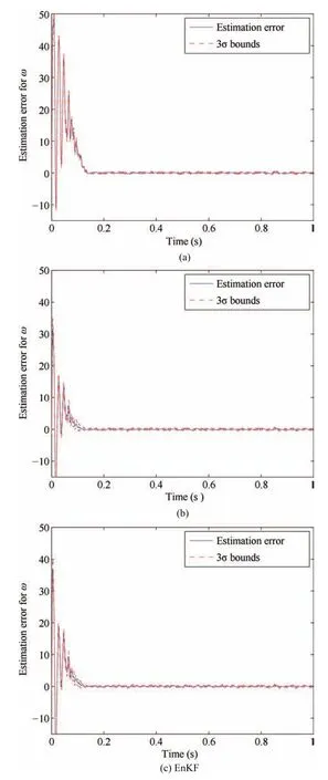
Fig.7.Estimation error for ω:(a)EKF;(b)UKF;(c)EnKF with Ns=100.

We draw the following remarks about nonlinear state estimation from our extensive simulations with this specific problem and experience with other problems in our past research.

1)The initial estimate can significantly impact the estimation accuracy.For the problem considered here,it is found that EKF and EnKF are more sensitive to an initial guess.It is noteworthy that an initial guess,if differing much from the truth,can lead to divergence of filters.Hence,one is encouraged to obtain a guess as close as possible to the truth by using prior knowledge or trying different guesses.

2)A filter’s performance can be problem-dependent.A filter can provide estimation at a decent accuracy when applied to a problem but may fail when used to handle another.Thus,the practitioners are suggested to try different filters whenever allowed to find out the one that performs the best for their specific problems.

3)Successful application of a filter usually requires to tune the covariance matrices and in some cases,parameters involved in a filter(e.g.,λ,αandβin UKF),because of their important influence on estimation[46].The trial-and-error method is common in practice.Meanwhile,there also exist some studies of systematic tuning methods,e.g.,[47],[48].Readers may refer to them for further information.

4)In choosing the best filter,engineers need to take into account all the factors relevant to the problem they are addressing,including but not limited to estimation accuracy,computational efficiency,system’s structural complexity,and problem size.To facilitate such a search,Table II summarizes the main differences and application areas of EKF,UKF and EnKF.

VII.OTHER FILTERING APPROACHES ANDESTIMATION PROBLEMS

Nonlinear stochastic estimation remains a major research challenge for the control research community.Continual research effort has been in progress toward the development of advanced methods and theories in addition to the KFs reviewed above.This section gives an overview of other major filtering approaches.

1)Gaussian Filters(GFs):GFs are a class of Bayesian filters enabled by a series of Gaussian distribution approximations.They bear much resemblance with KFs in view of their prediction-update structure and thus,in a broad sense,belong to the KF family.As seen earlier,the KF-based estimation relies on the evaluation of a set of integrals indeed,for example,the prediction ofxkis attained in(6)by computing the conditional mean off(xk-1)on Yk-1.The equation isrepeated here for convenience of reading:GFs approximatep(xk-1|Yk-1)with a Gaussian distribution having meanand covarianceNamely,is replaced by[33].Continuing with this approximation,one can use the Gaussian quadrature integration rules to evaluate the integral.A quadrature is a means of approximating a definite integral of a function by a weighted sum of values obtained by evaluating the function at a set of deterministic points in the domain of integration.An example of a one-dimensional Gaussian quadrature is the Gauss-Hermite quadrature,which plainly states that,for a given functiong(x),

TABLE IICOMPARISON OFEKF,UKFANDENKF

wheremis the number of points used,xifori=1,2,...,mthe roots of the Hermite polynomialHm(x),andwithe associated weights:

Exact equality holds for polynomials of order up to 2m-1.Applying the multivariate version of this quadrature,one can obtain a filter in a KF form,which is named Gauss-Hermite KF or GHKF[33],[49].GHKF reduces to UKF in certain cases[33].Besides,the cubature rules for numerical integration can also be used in favor of a KF realization,which yields a cubature KF(CKF)[50],[51].It is noteworthy that CKF is a special case of UKF givenα=1,β=0 andκ=0[52].

2)Gaussian-sum Filters(GSFs):Though used widely in the development of GFs and KFs,Gaussianity approximations are often inadequate and performance-limiting for many systems.To deal with a non-Gaussian PDF,GSFs represent it by a weighted sum of Gaussian basis functions[7].For instance,thea posterioriPDF ofxkis approximated by

3)Particle Filters(PFs):The PF approach was first proposed in the 1990’s[59]and came to prominence soon after that owing to its capacity for high-accuracy nonlinear non-Gaussian estimation.Today they have grown into a broad class of filters.As random-sampling-enabled numerical realizations of the Bayesian filtering principle,they are also referred to as the sequential Monte Carlo methods in the literature.Here,we introduce the essential idea with minimal statistical theory to offer the reader a flavor of this approach.Suppose thatNssamples,,are drawn fromp(xk-1|Yk-1)at timek-1.Theith sample is associated with a weightcan be empirically described as

This indicates that the estimate ofxk-1is

The samples can be propagated one-step forward to generate a sampling-based description ofxk,i.e.,

Then,an empirical sample-based distribution is built forp(xk|Yk)as in(62),and the estimate ofxkcan be computed as

In practical implementation of the above procedure,the issue of degeneracy may arise,which refers to the scenario that many or even most samples take almost zero weights.Any occurrence of degeneracy renders the affected samples useless.Remedying this situation requires the deployment of resampling,which replaces the samples by new ones drawn from the discrete empirical distribution defined by the weights.Summarizing the steps of sample propagation,weight update and resampling gives rise to a basic PF,which is schematically shown in Fig.8.While the above outlines a reasonably intuitive explanation of the PF approach,a rigorous development can be made on a solid statistical foundation,as detailed in[16],[60],[61].

Fig.8. A graphic diagram of the PF technique modified from[62].Suppose that a set of samples(particles,as shown in gray color in the figure)are used to approximate the conditional PDF of the state on the available measurements as a particle discrete distribution.A one-step-froward propagation is implemented to generate the samples for the state at the next time instant.On its arrival,the new measurement is used to update the weight of each sample to reflect its importance relative to others.Some samples may be given almost zero weight,referred to as degeneracy,and thus have meaningless contribution to the state estimation.Resampling is then performed to generate a new set of samples.

With the sample-based PDF approximation,PFs can demonstrate estimation accuracy superior to other filters given a sufficiently largeNs.It can be proven that their estimation error bound does not depend on the dimension of the system[63],implying applicability for high-dimensional systems.A possible limitation is their computational complexity,which comes atwithNs≫nx.Yet,a strong anticipation is that the rapid growth of computing power tends to overcome this limitation,enabling wider application of PFs.A plethora of research has also been undertaken toward computationally efficient PFs[64].A representative means is the Rao-Blackwellization that applies the standard KF to the linear part of a system and a PF to the nonlinear part and reduces the number of samples to operate on[16].The performance of PFs often relies on the quality of samples used.To this end,KFs can be used in combination to provide high-probability particles for PFs,leading to a series of combined KF-PF techniques[65]-[67].A recent advance is the implicit PF,which uses the implicit sampling method to generate samples capable of an improved approximation of the PDF[68],[69].

4)Moving-horizon Estimators(MHEs):They are an emerging estimation tool based on constrained optimization.In general,they aim to find the state estimate through minimizing a cost function subject to certain constraints.The cost function is formulated on the basis of the system’s behavior in a moving horizon.To demonstrate the idea,we consider the maximum a posteriori(MAP)estimation for the system in(1)during the horizon[k-N,k]as shown below:

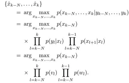
Assumingwk∼N(0,Q)andvk∼N(0,R)and using the logarithmic transformation,the above cost function becomes

where Φ(xk-N)is the arrival cost summarizing the past information up to the beginning of the horizon.The minimization here should be subject to the system model in(1).Meanwhile,some physically motivated constraints for the system behavior should be incorporated.This produces the formulation of MHE given as

where X,W and V are,respectively,the sets of all feasible values forx,wandvand imposed as constraints.It is seen

Fig.9.MHE performed over a moving observation horizon that spans N+1 time instants.For estimation at time k,the arrival cost Φ(xk-N)is determined first,which summarizes the information of the system behavior up to the beginning of the horizon.Then,the output measurements within the horizon,yk-N,...,yk,are used,along with the arrival cost,to conduct estimation ofˆxk-N,...,ˆxkthrough constrained optimization.

that MHE tackles the state estimation through constrained optimization executed over time in a receding-horizon manner,as shown in Fig.9.For an unconstrained linear system,MHE reduces to the standard KF.It is worth noting that the arrival cost Φ(xk-N)is crucial for the performance or even success of an MHE approach.In practice,an exact expression is often unavailable,thus requiring an approximation[70],[71].With the deployment of constrained optimization,MHE is computationally expensive and usually more suited for slow dynamic processes;however,the advancement of real-time optimization has brought some promises to its faster implementation[72],[73].

5)Simultaneous State and Parameter Estimation(SSPE):In state estimation problems,a system model is considered fully knowna priori.This may not be true in various real-world situations,where part or even all of the model parameters are unknown or subject to time-varying changes.Lack of knowledge of the parameters can disable an effort for state estimation in such a scenario.Hence,SSPE is motivated to enable state estimation self-adapting to the unknown parameters.A straightforward and popular way for SSPE is through state augmentation.To deal with the parameters,the state vector is augmented to include them,and on account of this,the state-space model is transformed accordingly to one with more dimensions.Then,a state estimation technique can be applied directly to the new model to estimate the augmented state vector,which is a joint estimation of the state variables and parameters.In the literature,EKF,UKF,EnKF and PFs have been modified using this idea for a broad range of applications[74]-[78].Another primary solution is the so-called dual Kalman filtering.By “dual”,it means that the state estimation and parameter estimation are performed in parallel and alternately.As such,the state estimate is used to estimate the parameters,and the parameter estimate is used to update the state estimation.Proceeding with this idea,EKF,UKF and EnKF can be dualized[79]-[82].It should be pointed out that caution should be taken when an SSPE approach is developed.Almost any SSPE problem is nonlinear by nature due to coupling between state variables and parameters.The joint state observability and parameter identifiability may be unavailable,or the estimation may get stuck in local minima.Consequently,the convergence can be vulnerable or unguaranteed,diminishing the chance of successful estimation.Thus application-specific SSPE analysis and development are recommended.

6)Simultaneous State and Input Estimation(SSIE):Some practical applications entail not only unknown states but also unknown inputs.An example is the operation monitoring for an industrial system subject to unknown disturbance,where the operational status is the state and the disturbance the input.In maneuvering target tracking,the tracker often wants to estimate the state of the target,e.g.,position and velocity,and the input,e.g.,the acceleration.Another example is the wild fire data assimilation extensively investigated in the literature.The spread of wild fire is often driven by local meteorological conditions such as the wind.This gives rise to the need for a joint estimation of both the fire perimeters(state)and the wind speed(input)toward accurate monitoring of the fire growth.

The significance of SSIE has motivated a large body of work.A lead was taken in[83]with the development of a KF-based approach to estimate the state and external white process noise of a linear discrete-time system.Most recent research builds on the existing state estimation techniques.Among them,we highlight KF[84],[85],MHE[86],H∞- filtering[87],sliding mode observers[88],[89],and minimum-variance unbiased estimation[90]-[94].SSIE for nonlinear systems involves more complexity,with fewer results reported.In[95],[96],SSIE is investigated for a special class of nonlinear systems that consist of a nominally linear part and a nonlinear part.However,the Bayesian statistical thinking has been generalized to address this topic,exemplifying its power in the development of nonlinear SSIE approaches.In[97],[98],a Bayesian approach along with numerical optimization is taken to achieve SSIE for nonlinear systems of a general form.This Bayesian approach is further extended in[99],[100]to build an ensemble-based SSIE method,as a counterpart of EnKF,for high-dimensional nonlinear systems.It is noteworthy that SSIE and SSPE would overlap if we consider the parameters as a special kind of inputs to the system.In this case,the SSIE approaches may find their use in solving SSPE problems.

VIII.CONCLUSION

This article offers a state-of-the-art review of nonlinear state estimation approaches.As a fundamental problem encountered across a few research areas,nonlinear stochastic estimation has stimulated a sustaining interest during the past decades.In the pursuit of solutions,the Bayesian analysis has proven to be a time-tested and powerful methodology for addressing various types of problems.In this article,we first introduce the Bayesian thinking for nonlinear state estimation,showing the nature of state estimation from the perceptive of Bayesian update.Based on the notion of Bayesian state estimation,a general form of the celebrated KF is derived.Then,we illustrate the development of the standard KF for linear systems and EKF,UKF and EnKF for nonlinear systems.A case study of state estimation for speed-sensorless induction motors is provided to present a comparison of the EKF,UKF and EnKF approaches.We further extend our view to a broader horizon including GF,GSF,PF and MHE approaches,which are also deeply rooted in the Bayesian state estimation and thus can be studied from a unified Bayesian perspective to a large extent.

Despite remarkable progress made thus far,it is anticipated that nonlinear Bayesian estimation continues to see intensive research in the coming decades.This trend is partially driven by the need to use state estimation as a mathematical tool to enable various emerging systems in contemporary industry and society,stretching from autonomous transportation to sustainable energy and smart X(grid,city,planet,geosciences,etc.).Here,we envision several directions that may shape the future research in this area.The first one lies in accurately characterizing the result of a nonlinear transformation applied to a probability distribution.Many of the present methods such as EKF,UKF and EnKF were more or less motivated to address this fundamental challenge.However,there still exists no solution universally acknowledged as being satisfactory,leaving room for further exploration.Second,much research is needed to deal with uncertainty.Uncertainty is intrinsic to many practical systems because of unmodeled dynamics,external disturbances,inherent variability of a dynamic process,and sensor noise,representing a major threat to successful estimation.Although the literature contains many results on state estimation robust to uncertainty,the research has not reached a level of maturity because of the difficulty involved.A third research direction is optimal sensing structure design.Sensing structure or sensor deployment is critical for data informativeness and thus can significantly affect the effectiveness of estimation.An important question thus is how to achieve co-design of a sensing structure and Bayesian estimation approach to maximize estimation accuracy.Fourth,Bayesian estimation in a cyber-physical setting is an imperative.Standing at the convergence of computing,communication and control,cyber-physical systems(CPSs)are foundationally important and underpinning today’s smart X initiatives[101],[102].They also present new challenges for estimation,which include communication constraints or failures,computing limitations,and cyber data attacks.The current research is particularly rare on nonlinear Bayesian estimation for CPSs.Finally,many emerging industrial and social applications are data-intensive,thus asking for a seamless integration of Bayesian estimation with big data processing algorithms.New principles,approaches and computing tools must be developed to meet this pressing need,which should make an unprecedented opportunity to advance the Bayesian estimation theory and applications.

APPENDIX

This appendix offers a summary of the properties of the Gaussian distribution.Suppose thatz∈Rnis a Gaussian random vector withz∼N(¯z,Pz).The PDF ofzis expressed as

Some useful properties of the Gaussian vectors are as follows[103].

1)

2)The af fine transformation ofz,Az+b,is Gaussian,i.e.,

3)The sum of two independent Gaussian random vectors is Gaussian;i.e.,ifz1∼N(¯z1,Pz1)andz2∼N(¯z2,Pz2)and ifz1andz2are independent,then

4)For two random vectors jointly Gaussian,the conditional distribution of one given the other is Gaussian.Specifically,ifz1andz2are jointly Gaussian with

[1]Late Rev.Mr.Bayes,and F.R.S,“LII.An essay towards solving a problem in the doctrine of chances.By the Late Rev.Mr.Bayes,F.R.S.Communicated by Mr.Price,in a Letter to John Canton,A.M.F.R.S,”Phil.Trans.,vol.53,pp.370-418,Jan.1763.

[2]A.I.Dale,“Bayes or Laplace?An examination of the origin and early applications of Bayes’theorem,”Arch.Hist.Exact Sci.,vol.27,no.1,pp.23-47,Mar.1982.

[3]D.Malakoff,“Bayes offers a ‘new’way to make sense of numbers,”Science,vol.286,no.5444,pp.1460-1464,Nov.1999.

[4]A.Jackson,“Kalman receives national medal of science,”Not.AMS,vol.57,no.1,pp.56-57,Jan.2010.

[5]R.E.Kalman,“A new approach to linear filtering and prediction problems,”J.Basic Eng.,vol.82,no.1,pp.35-45,Mar.1960.

[6]Y.Ho and R.Lee,“A Bayesian approach to problems in stochastic estimation and control,”IEEE Trans.Automat.Control,vol.9,no.4,pp.333-339,Oct.1964.

[7]B.D.O.Anderson and J.B.Moore,Optimal Filtering.Englewood Cliffs:Prentice-Hall,1979.

[8]Wikipedia Contributors,“Kalman filterg-Wikipedia,the free encyclopedia,”[Online].Available:https://en.wikipedia.org/wiki/Kalman filterg.

[9]F.Auger,M.Hilairet,J.M.Guerrero,E.Monmasson,T.Orlowska-Kowalska,and S.Katsura,“Industrial applications of the Kalman filter:A review,”IEEE Trans.Ind.Electron.,vol.60,no.12,pp.5458-5471,Dec.2013.

[10]M.Boutayeb,H.Rafaralahy,and M.Darouach,“Convergence analysis of the extended Kalman filter used as an observer for nonlinear deterministic discrete-time systems,”IEEE Trans.Automat.Control,vol.42,no.4,pp.581-586,Apr.1997.

[11]A.J.Krener, “The convergence of the extended Kalman filter,”inDirections in Mathematical Systems Theory and Optimization,A.Rantzer and C.Byrnes,Eds.Berlin,Heidelberg:Springer,2003,vol.286,pp.173-182.

[12]S.Kluge,K.Reif,and M.Brokate,“Stochastic stability of the extended Kalman filter with intermittent observations,”IEEE Trans.Automat.Control,vol.55,no.2,pp.514-518,Feb.2010.

[13]S.Bonnabel and J.J.Slotine,“A contraction theory-based analysis of the stability of the deterministic extended Kalman filter,”IEEE Trans.Automat.Control,vol.60,no.2,pp.565-569,Feb.2015.

[14]A.Barrau and S.Bonnabel,“The invariant extended Kalman filter as a stable observer,”IEEE Trans.Automat.Control,vol.62,no.4,pp.1797-1812,Apr.2017.

[15]H.Tanizaki,Nonlinear Filters:Estimation and Applications.Berlin Heidelberg:Springer-Verlag,1996.

[16]S.Sa¨rkka¨,Bayesian Filtering and Smoothing.Cambridge:Cambridge University Press,2013.

[17]M.Roth and F.Gustafsson,“An efficient implementation of the second order extended Kalman filter,”inProc.14th Int.Conf.Information Fusion(FUSION),Chicago,IL,USA,pp.1-6,2011.

[18]A.H.Jazwinski,Stochastic Processes and Filtering Theory.New York:Academic Press,1970.

[19]B.M.Bell and F.W.Cathey,“The iterated Kalman filter update as a gauss-newton method,”IEEE Trans.Automat.Control,vol.38,no.2,pp.294-297,Feb.1993.

[20]S.J.Julier,J.K.Uhlmann,and H.F.Durrant-Whyte,“A new approach for filtering nonlinear systems,”inProc.1995 American Control Conf.,vol.3,Seattle,WA,USA,pp.1628-1632,1995.

[21]S.J.Julier and J.K.Uhlmann,“A new extension of the Kalman filter to nonlinear systems,”inProc.AeroSense:The 11th International Symp.Aerospace/Defence Sensing,Simulation and Controls,Orlando,FL,USA,pp.182-193,1997.

[22]S.J.Julier and J.K.Uhlmann,“Unscented filtering and nonlinear estimation,”Proc.IEEE,vol.92,no.3,pp.401-422,2004.

[23]E.Wan and R.van der Merwe, “The unscencted Kalman filter,”inKalman Filtering and Neural Networks,S.Haykin,Ed.New York:John Wiley&Sons,2001,pp.221-269.

[24]H.M.T.Menegaz,J.Y.Ishihara,G.A.Borges,and A.N.Vargas,“A systematization of the unscented Kalman filter theory,”IEEE Trans.Automat.Control,vol.60,no.10,pp.2583-2598,Oct.2015.

[25]R.Van Der Merwe and E.A.Wan,“The square-root unscented Kalman filter for state and parameter-estimation,”inProc.IEEE Int.Conf.Acoustics,Speech,and Signal Processing,vol.6,Salt Lake City,UT,USA,pp.3461-3464,2001.

[26]S.J.Julier,“The spherical simplex unscented transformation,”inProc.American Control Conf.,vol.3,Denver,CO,USA,pp.2430-2434,2003.

[27]W.C.Li,P.Wei,and X.C.Xiao,“A novel simplex unscented transform and filter,”inProc.Int.Symp.Communications and Information Technologies,Sydney,Australia,pp.926-931,2007.

[28]K.Ponomareva,P.Date,and Z.D.Wang,“A new unscented Kalman filter with higher order moment-matching,”inProc.19th Int.Symp.Mathematical Theory of Networks and Systems,Budapest,Hungary,pp.1609-1613,2010.

[29]A.C.Charalampidis and G.P.Papavassilopoulos,“Development and numerical investigation of new non-linear Kalman filter variants,”IET Control Theory Appl.,vol.5,no.10,pp.1155-1166,Aug.2011.

[30]J.Dunik,M.Simandl,and O.Straka,“Unscented Kalman filter:Aspects and adaptive setting of scaling parameter,”IEEE Trans.Automat.Control,vol.57,no.9,pp.2411-2416,Sep.2012.

[31]J.L.Crassidis,“Sigma-point Kalman filtering for integrated GPS and inertial navigation,”IEEE Trans.Aerosp.Electron.Syst.,vol.42,no.2,pp.750-756,Apr.2006.

[32]R.van der Merwe,“Sigma-point Kalman filters for probabilistic inference in dynamic state-space models,”Ph.D.dissertation,Oregon Health&Science University,2004.

[33]K.Ito and K.Xiong,“Gaussian filters for nonlinear filtering problems,”IEEE Trans.Automat.Control,vol.45,no.5,pp.910-927,May 2000.

[34]G.Evensen,“Sequential data assimilation with a nonlinear quasi-geostrophic model using Monte Carlo methods to forecast error statistics,”J.Geophys.Res.:Oceans,vol.99,no.C5,pp.10143-10162,May 1994.

[35]G.Evensen and P.J.van Leeuwen,“Assimilation of geosat altimeter data for the agulhas current using the ensemble Kalman filter with a quasigeostrophic model,”Mon.Wea.Rev.,vol.124,pp.85-96,Jan.1996.

[36]P.L.Houtekamer and H.L.Mitchell,“Data assimilation using an ensemble Kalman filter technique,”Mon.Wea.Rev.,vol.126,pp.796-811,Mar.1998.

[37]J.Mandel, “Efficient implementation of the ensemble Kalman filter,”University of Colorado at Denver,Tech.Rep.UCDHSC/CCM Report No.231,2006.

[38]S.Lakshmivarahan and D.J.Stensrud,“Ensemble Kalman filter,”IEEE Control Syst.,vol.29,no.3,pp.34-46,Jun.2009.

[39]G.Evensen,Data Assimilation:The Ensemble Kalman Filter,2nd ed.Berlin Heidelberg:Springer,2009.

[40]J.Mandel,L.Cobb,and J.D.Beezley,“On the convergence of the ensemble Kalman filter,”Appl.Math.,vol.56,no.6,pp.533-541,Dec.2011.

[41]M.Montanari,S.M.Peresada,C.Rossi,and A.Tilli,“Speed sensorless control of induction motors based on a reduced-order adaptive observer,”IEEE Trans.Control Syst.Technol.,vol.15,no.6,pp.1049-1064,Nov.2007.

[42]S.R.Bowes,A.Sevinc,and D.Holliday,“New natural observer applied to speed-sensorless dc servo and induction motors,”IEEE Trans.Ind.Electron.,vol.51,no.5,pp.1025-1032,Oct.2004.

[43]R.Marino,P.Tomei,and C.M.Verrelli,“A global tracking control for speed-sensorless induction motors,”Automatica,vol.40,no.6,pp.1071-1077,Jun.2004.

[44]Y.B.Wang,L.Zhou,S.A.Bortoff,A.Satake,and S.Furutani,“High gain observer for speed-sensorless motor drives:algorithm and experiments,”inProc.IEEE Int.Conf.Advanced Intelligent Mechatronics,Banff,AB,UK,pp.1127-1132,2016.

[45]L.Zhou and Y.B.Wang,“Speed sensorless state estimation for induction motors:a moving horizon approach,”inProc.American Control Conf.,Boston,MA,USA,pp.2229-2234,2016.

[46]Q.B.Ge,T.Shao,Z.S.Duan,and C.L.Wen,“Performance analysis of the Kalman filter with mismatched noise covariances,”IEEE Trans.Automat.Control,vol.61,no.12,pp.4014-4019,Dec.2016.

[47]L.A.Scardua and J.J.da Cruz,“Complete of fl ine tuning of the unscented kalman filter,”Automatica,vol.80,pp.54-61,Jun.2017.

[48]B.F.La Scala,R.R.Bitmead,and B.G.Quinn,“An extended Kalman filter frequency tracker for high-noise environments,”IEEE Trans.Signal Process.,vol.44,no.2,pp.431-434,Feb.1996.

[49]B.Jia,M.Xin,and Y.Cheng,“Sparse Gauss-Hermite quadrature filter with application to spacecraft attitude estimation,”J.Guid.Control Dyn.,vol.34,no.2,pp.367-379,Mar.-Apr.2011.

[50]I.Arasaratnam and S.Haykin,“Cubature Kalman filters,”IEEE Trans.Automat.Control,vol.54,no.6,pp.1254-1269,Jun.2009.

[51]B.Jia,M.Xin,and Y.Cheng, “High-degree cubature Kalman filter,”Automatica,vol.49,no.2,pp.510-518,Feb.2013.

[52]S.Sa¨rkka¨,J.Hartikainen,L.Svensson,and F.Sandblom.On the relation between Gaussian process quadratures and sigma-point methods.arXiv:1504.05994,2015.

[53]J.Park and I.W.Sandberg,“Universal approximation using radialbasis-function networks,”Neural Comput.,vol.3,no.2,pp.246-257,Jun.1991.

[54]O.Straka,J.Dun´ık,and M.Simandl, “Gaussian sum unscented Kalman filter with adaptive scaling parameters,”inProc.14th Int.Conf.Information Fusion,Chicago,IL,USA,pp.1-8,2011.

[55]L.Dovera and E.Della Rossa,“Multimodal ensemble Kalman filtering using Gaussian mixture models,”Computat.Geosci.,vol.15,no.2,pp.307-323,Mar.2011.

[56]J.T.Horwood and A.B.Poore,“Adaptive Gaussian sum filters for space surveillance,”IEEE Trans.Automat.Control,vol.56,no.8,pp.1777-1790,Aug.2011.

[57]J.H.Kotecha and P.M.Djuric,“Gaussian sum particle filtering,”IEEE Trans.Signal Process.,vol.51,no.10,pp.2602-2612,Oct.2003.

[58]G.Terejanu,P.Singla,T.Singh,and P.D.Scott,“Adaptive Gaussian sum filter for nonlinear Bayesian estimation,”IEEE Trans.Automat.Control,vol.56,no.9,pp.2151-2156,Sep.2011.

[59]N.J.Gordon,D.J.Salmond,and A.F.M.Smith,“Novel approach to nonlinear/non-Gaussian Bayesian state estimation,”IEE Proc.F:Radar Signal Process.,vol.140,no.2,pp.107-113,Apr.1993.

[60]A.Doucet and A.M.Johansen,“A tutorial on particle filtering and smoothing: fifteen years later,”inThe Oxford Handbook of Nonlinear Filtering,D.Crisan and B.Rozovskiˇi,Eds.Oxford:Oxford University Press,pp.656-704,2011.

[61]M.S.Arulampalam,S.Maskell,N.Gordon,and T.Clapp,“A tutorial on particle filters for online nonlinear/non-Gaussian Bayesian tracking,”IEEE Trans.Signal Process.,vol.50,no.2,pp.174-188,Feb.2002.[62]A.Parker,“Dealing with data overload in the scientific realm,”Science and Technology Review,4-11,2013.[Online].Avaliable:https://str.llnl.gov/content/pages/january-2013/pdf/01.13.1.pdf

[63]D.Crisan and A.Doucet,“Convergence of sequential Monte Carlo methods,”Technical Report,University of Cambridge,2000.

[64]W.Yi,M.R.Morelande,L.J.Kong,and J.Y.Yang,“A computationally efficient particle filter for multitarget tracking using an independence approximation,”IEEE Trans.Signal Process.,vol.61,no.4,pp.843-856,Feb.2013.

[65]F.J.F.G.de Freitas,M.Niranjan,A.H.Gee,and A.Doucet,“Sequential monte carlo methods to train neural network models,”Neural Comput.,vol.12,no.4,pp.955-993,Apr.2000.

[66]R.van der Merwe,A.Doucet,N.de Freitas,and E.Wan,“The unscented particle filter,”inAdvances in Neural Information Processing Systems 13,Cambridge,CA,USA,pp.584-590,2001.

[67]L.Q.Li,H.B.Ji,and J.H.Luo,“The iterated extended Kalman particle filter,”inProc.IEEE Int.Symp.Communications and Information Technology,vol.2,Beijing,China,pp.1213-1216,2005.

[68]A.J.Chorin and X.M.Tu, “Implicit sampling for particle filters,”Proc.Natl.Acad.Sci.USA,vol.106,no.41,pp.17429-17254,Oct.2009.

[69]A.Chorin,M.Morzfeld,and X.M.Tu,“Implicit particle filters for data assimilation,”Commun.Appl.Math.Comput.Sci.,vol.5,no.2,pp.221-240,Nov.2010.

[70]C.V.Rao,J.B.Rawlings,and D.Q.Mayne,“Constrained state estimation for nonlinear discrete-time systems:stability and moving horizon approximations,”IEEE Trans.Automat.Control,vol.48,no.2,pp.246-258,Feb.2003.

[71]C.V.Rao,“Moving horizon strategies for the constrained monitoring and control of nonlinear discrete-time systems,”Ph.D.dissertation,University of Wisconsin Madison,2000.

[72]M.J.Tenny and J.B.Rawlings,“Efficient moving horizon estimation and nonlinear model predictive control,”inProc.2002 American Control Conf.,vol.6,Anchorage,AK,USA,pp.4475-4480,2002.

[73]M.Diehl,H.J.Ferreau,and N.Haverbeke,“Efficient numerical methods for nonlinear mpc and moving horizon estimation,”inNonlinear Model Predictive Control,L.Magni,D.M.Raimondo,and F.Allgo¨wer,Eds.Berlin Heidelberg:Springer,vol.384,pp.391-417,2009.

[74]J.Ching,J.L.Beck,and K.A.Porter,“Bayesian state and parameter estimation of uncertain dynamical systems,”Probabilist.Eng.Mech.,vol.21,no.1,pp.81-96,Jan.2006.

[75]H.Z.Fang,Y.B.Wang,Z.Sahinoglu,T.Wada,and S.Hara,“Adaptive estimation of state of charge for lithium-ion batteries,”inProc.American Control Conf.,Washington,DC,USA,pp.3485-3491,2013.

[76]H.Z.Fang,Y.B.Wang,Z.Sahinoglu,T.Wada,and S.Hara,“State of charge estimation for lithium-ion batteries:an adaptive approach,”Control Eng.Pract.,vol.25,pp.45-54,Apr.2014.

[77]G.Chowdhary and R.Jategaonkar,“Aerodynamic parameter estimation from fl ight data applying extended and unscented Kalman filter,”Aerosp.Sci.Technol.,vol.14,no.2,pp.106-117,Mar.2010.

[78]T.Chen,J.Morris,and E.Martin,“Particle filters for state and parameter estimation in batch processes,”J.Process Control,vol.15,no.6,pp.665-673,Sep.2005.

[79]E.A.Wan and A.T.Nelson, “Dual extended Kalman filter methods,”inKalman Filtering and Neural Networks,S.Haykin,Ed.New York:John Wiley&Sons,Inc.,pp.123-173,2001.

[80]E.A.Wan,R.Van Der Merwe,and A.T.Nelson,“Dual estimation and the unscented transformation,”inProc.12th Int.Conf.Neural Information Processing Systems,Denver,CO,2000,USA,pp.666-672.

[81]M.C.VanDyke,J.L.Schwartz,and C.D.Hall,“Unscented Kalman filtering for spacecraft attitude state and parameter estimation,”inProc.AAS/AIAA Space Flight Mechanics Conf.,Maui,Hawaii,USA,2004.[82]H.Moradkhani,S.Sorooshian,H.V.Gupta,and P.R.Houser,“Dual state-parameter estimation of hydrological models using ensemble Kalman filter,”Adv.Water Resour.,vol.28,no.2,pp.135-147,Feb.2005.

[83]J.Mendel,“White-noise estimators for seismic data processing in oil exploration,”IEEE Trans.Automat.Control,vol.22,no.5,pp.694-706,Oct.1977.

[84]C.S.Hsieh,“Robust two-stage Kalman filters for systems with unknown inputs,”IEEE Trans.Automat.Control,vol.45,no.12,pp.2374-2378,Dec.2000.

[85]C.S.Hsieh,“On the optimality of two-stage Kalman filtering for systems with unknown inputs,”Asian J.Control,vol.12,no.4,pp.510-523,Jul.2010.

[86]L.Pina and M.A.Botto,“Simultaneous state and input estimation of hybrid systems with unknown inputs,”Automatica,vol.42,no.5,pp.755-762,May 2006.

[87]F.Q.You,F.L.Wang,and S.P.Guan,“Hybrid estimation of state and input for linear discrete time-varying systems:a game theory approach,”Acta Automatica Sinica,vol.34,no.6,pp.665-669,Jun.2008.

[88]T.Floquet,C.Edwards,and S.K.Spurgeon,“On sliding mode observers for systems with unknown inputs,”Int.J.Adapt.Control Signal Process.,vol.21,no.8-9,pp.638-656,Oct.-Nov.2007.

[89]F.J.Bejarano,L.Fridman,and A.Poznyak,“Exact state estimation for linear systems with unknown inputs based on hierarchical supertwisting algorithm,”Int.J.Robust Nonlinear Control,vol.17,no.18,pp.1734-1753,Dec.2007.

[90]S.Gillijns and B.De Moor,“Unbiased minimum-variance input and state estimation for linear discrete-time systems with direct feedthrough,”Automatica,vol.43,no.5,pp.934-937,May 2007.

[91]S.Gillijns and B.De Moor,“Unbiased minimum-variance input and state estimation for linear discrete-time systems,”Automatica,vol.43,no.1,pp.111-116,Jan.2007.

[92]H.Z.Fang,Y.Shi,and J.Yi,“A new algorithm for simultaneous input and state estimation,”inProc.American Control Conf.,Seattle,WA,USA,pp.2421-2426,2008.

[93]H.Z.Fang,Y.Shi,and J.Yi,“On stable simultaneous input and state estimation for discrete-time linear systems,”Int.J.Adapt.Control Signal Process.,vol.25,no.8,pp.671-686,Aug.2011.

[94]H.Z.Fang and R.A.de Callafon,“On the asymptotic stability of minimum-variance unbiased input and state estimation,”Automatica,vol.48,no.12,pp.3183-3186,Dec.2012.

[95]M.Corless and J.Tu,“State and input estimation for a class of uncertain systems,”Automatica,vol.34,no.6,pp.757-764,Jun.1998.

[96]Q.P.Ha and H.Trinh,“State and input simultaneous estimation for a class of nonlinear systems,”Automatica,vol.40,no.10,pp.1779-1785,Oct.2004.

[97]H.Z.Fang,R.A.de Callafon,and J.Corte´s,“Simultaneous input and state estimation for nonlinear systems with applications to flow field estimation,”Automatica,vol.49,no.9,pp.2805-2812,Sep.2013.

[98]H.Z.Fang,R.A.de Callafon,and P.J.S.Franks,“Smoothed estimation of unknown inputs and states in dynamic systems with application to oceanic flow field reconstruction,”Int.J.Adapt.Control Signal Process.,vol.29,no.10,pp.1224-1242,Oct.2015.

[99]H.Z.Fang and R.A.de Callafon,“Simultaneous input and state if ltering:an ensemble approach,”inProc.IEEE 54th Conf.Decision and Control(CDC),Osaka,Japan,pp.437-442,2015.

[100]H.Z.Fang,T.Srivas,R.A.de Callafon,and M.A.Haile,“Ensemblebased simultaneous input and state estimation for nonlinear dynamic systems with application to wild fire data assimilation,”Control Eng.Pract.,vol.63,pp.104-115,Jun.2017.

[101]Y.Liu,Y.Peng,B.L.Wang,S.R.Yao,and Z.H.Liu,“Review on cyber-physical systems,”IEEE/CAA J.Autom.Sinica,vol.4,no.1,pp.27-40,Jan.2017.

[102]X.Guan,B.Yang,C.Chen,W.Dai,and Y.Wang,“A comprehensive overview of cyber-physical systems:from perspective of feedback system,”IEEE/CAA J.Autom.Sinica,vol.3,no.1,pp.1-14,2016.

[103]J.V.Candy,Bayesian Signal Processing:Classical,Modern and Particle Filtering Methods.New York,NY,USA:Wiley-Interscience,2009.