Heat and work in Markovian quantum master equations:concepts,fluctuation theorems,and computations

Fei Liu

School of Physics and Nuclear Energy Engineering,Beihang University,Beijing 100191,China

I.INTRODUCTION

In the past two decades,there has been growing interest[1−44]in the stochastic heat and work of nonequilibrium quantum processes.These studies include investigations of the definitions of these fundamental thermodynamic quantities,their statistical characteristics in general or specific physical models,computational methods,and experimental measurements and realizations.This research boom is driven mainly by two causes.One cause is the practical possibility of manipulating and controlling small quantum systems[45−49].Energy,one of the most important physical quantities,and its transfer are always of great concern,while randomness is an intrinsic characteristic of quantum systems.The other motivation is from theoretical interests.Over almost the same period,a breakthrough in non-equilibrium physics was the discovery of a variety offluctuation theorems(FTs)[50−61].These formulas concerning heat,work,and total entropy production were proved to be exact even in far-from-equilibrium regions,whereas in near-equilibrium regions,they are usually reduced to the famousfluctuation-dissipation theorems[62−64].Because these remarkable results were usually obtained in classical physical systems,there has been intensive theoretical interest to extend them into the quantum regime[48,50,65−73].

Among these theoretical efforts,quantum systems that can be described by Markovian quantum master equations(MQMEs)have attracted considerable attention[1−8,10−27,29,30,36,39,41,74].We believe that this is not coincidental.On the one hand,as the closest extension of Hamiltonian systems,MQMEs[75−77]have solid mathematical and physical foundations[78−80].On the other hand,in the statistical physics community,there has long been a tradition of studying irreversible thermodynamics using the MQMEs[47,81−87].Mukamel[1]proved a quantum Jarzynski equality(JE)for specific MQMEs that can be transformed to the classic MEs[57,88,89]in the adiabatic basis.He also presented a formal analogy between the JE and the dephasing of quantum coherences in spectral line shapes.Using an analogous idea,for general Lindblad-type QMEs,Esposito and Mukamel[6]obtained several FTs by recasting these equations into the classical birth-death MEs in a time-dependent basis that diagonalizes the reduced density matrix of the system.These authors then unraveled these MEs by classical stochastic jump processes and called them quantum trajectories.Although Esposito and Mukamel defined heat and work at these quantum trajectories as done in the classical cases[59,89],the relations of these trajectories to measurement scheme remain unclear[90,91].Additionally,to establish a quantum JE,De Roeck and Maes defined the quantum history of a subsystem(they called the subsystem and heat bath the total system)[2].A realization in their paper is a repeated discrete projective measurement on an open quantum system;between two successive measurements,the subsystem is weakly coupled to an infinite free reservoir and is subjected to an external time-dependent driving potential varying on the time scale of dissipation.After that,De Roeck and Maes[92],De Roeck[3],and Derezinski et al[93]systematically investigated the quantum extension of the Callavotti-Cohen FT for entropy production[52].Their results showed that this task could be realized either in microscopic Hamiltonian systems or in time-homogenous Lindblad QME with a stationary state.Importantly,the former was rigorously proved to converge to the latter in the weak-coupling limit.The important ingredients in defining the entropy production of the specific MQMEs are to unravel them into quantum jump trajectories(QJTs)[78,94−99],to give probability measures on these trajectories and to interpret thefluctuating heat current as energy quanta that are transferred between the subsystem and reservoirs.Note that the QJTs here are not the same as those unravelled from the classical MEs as Espositor and Mukamel used[6].Interestingly,Breuer[100]independently defined the same heat current when he investigated the entropy production rate of the stochastic state vector dynamics.For Hamiltonian systems,heat was microscopically defined as energy eigenvalue differences between the reservoirs at the end and beginning of non-equilibrium processes.This is the famous two-energy-measurement(TEM)scheme defining stochastic thermodynamic quantities[65].Talkner et al.[8]proved that JE is always true for general open quantum systems if the system weakly interacts with its environment.In their paper,work was microscopically defined as energy eigenvalue differences between the composite system and its environment at the end and beginning of non-equilibrium processes.Their conclusion does not depend on whether the dynamics of the system is Markovian.Although MQMEs are typical open systems and fulfill the weakly coupling condition,since additional approximations are involved in these equations,whether the strong statement given by Talkner et al.remains true in these equations is not very clear.Crooks[101]discussed how to express the JE for open quantum systems whose dynamics can be described by general quantum dynamical semigroups[78].To concisely represent the measurements of the heatflow from environment to the systems,a Hermitian map superoperator was used.In his another paper,Crooks[7]defined the time reversal of a quantum dynamical semigroup having a positive-definite invariant state.At arbitrary time the dynamical semigroup is a completely positive,trace-preserving(CPTP)quantum map,and the map admits a operator-sum representation in terms of a collection of Kraus operators.Because each Kraus operator represents an interaction with the environment that may be measured and recorded by an external observer,Crooks defined a quantum history by noting the observed sequence of Kraus operators.Under these two definitions,Crooks found that the probability of a quantum history and that of the time-reversed history are related by the heat exchanged with the environment.This very insightful paper was further generalized by Manzano et al.[23]recently,and a very general FT was obtained.

The reader might note that the above studies were mainly concerned with the validity of various quantum FTs,and their considerations were usually abstract.This situation remained unchanged until Esposito et al.[4]derived a generalized quantum master equation(GQME)that can concretely calculate the characteristic function(CF,or the generating function in their paper)of a heat or matter current in time-homogenous MQMEs.The heat or matter current therein was also defined by the TEM scheme on the reservoirs.Importantly,the statistics of these stochastic quantities were implied in the GQME and its solution.This key equation quickly became popular in the literature.For instance,Silaev et al.[18]used the GQME to investigate the work and heat statistics in weakly driven open quantum systems[80].Gasparinetti et al[24]and Cuetara et al.[25]further extended the idea of Esposito et al.to periodically driven MQMEs[102−105].A very analogous GQME was derived as well.Garrahan and his coauthors[31,32,106−108]applied the largedeviation method[109]to study the “thermodynamics”of the QJTs of Lindblad QMEs,e.g.,the dynamical crossover and dynamical phase transitions.Their discussions were also based on the GQME.In one of their papers,Garrahan and Lesanovsky[31]noted that the GQME has been in the literature of quantum optics for a long time[97].However,in contrast to what Esposito et.al[4]did,the earlier version was based on the concept of QJTs and was obtained byfinding a set of evolution equations for the reduced density matrix with given jump events[110,111].Hence,their observation could be thought of as a concrete demonstration of the statement given by Derezinski et al.[93].Horowitz[10]formulated heat and work for the QJTs of a continuously monitored forced harmonic oscillator coupled to a thermal reservoir.A detailed FT for QJTs was derived.In contrast to previous results using QJTs[31−92],in his model,the Hamiltonian is time dependent.In the same spirit,Hekking and Pelako[14]investigated the statistics of work for the QJTs in a weakly driven twolevel system coupled to a heat reservoir.They calculated the work distributions of the simple model and proved a quantum JE.Horowitz and Parrondom[5]and Horowitz and Sagawa[112]studied the quantum adiabatic and non-adiabatic entropy productions for the general Lindblad master equations.A quantum dual process analogous to the classical dual Markov process[113]was defined by these authors.They found that these two entropy productions could be defined as ratios of the probabilities of QJTs in the original and dual processes.Chetrite and Mallick[12]obtained a quantum Jarzynski-Hatano-Sasa equality for a general Lindblad equation having an instantaneous stationary state solution.To prove this result,they introduced a modified Lindblad equation and utilized a quantum Feynman-Kac(FK)formula[11].Their results were abstract and lacked probability interpretations.We[16,17]noted that,in weakly driven and adiabatically driven MQMEs,the quantum FK formula was a book-keeping expression of the moment-generating function for work;it has a probability explanation if applying the measure of the QJTs.Additionally,in these two papers,in addition to proving a Bochkov-Kuzovlev equality(BKE)and JE,we presented two CF methods for calculating the exclusive and inclusive work distributions[114,115].These equations are very analogous to those utilized in classical stochastic systems[116,117].We[118]studied whether the CF of the exclusive work is equivalent to the CF based on the TEM work defined on the composite system and heat reservoir[69,115].This affirmative result further stimulated us[119]to develop the CF methods of heat and work based on the QJT concept for several time-dependent MQMEs.Their connections with the CFs of heat and work based on the TEM scheme were established as well.Very recently,Suomela et al.[21,22]developed a modified QJT model for systems interacting with afinite-size heat bath.This work was mainly motivated by a calorimetric measurement of work in driven open quantum system[120].Elouard et al.[41]considered the possibility of defining quantum heat that is purely measurement induced.In addition to QJTs,their formalism also includes the quantum sate diffusion(QSD)unravelling of MQMEs.Finally,Gong et al.[27]considered these feedback effects on quantum fluctuation effects using the QJT concept.

After the above long sketch of the literature,we clearly see that two main strategies are emerging in the studies of the quantum stochastic thermodynamics(QST)of MQMEs.One strategy is based on the TEM scheme defining thermodynamic quantities on the composite system and environments[4,65,71,92];the basic tool of computations and statistical analysis is the GQME[4,18,24,25].The other strategy is to utilize the fact that the MQMEs can be unraveled into QJT-s[78,94−99];along each QJT,heat,work,and entropy production can be well defined[10,14,16,17,92,100];the computational and statistical analysis method could be straightforward Monte-Carlo simulation[10,14]or the CFs based on the QJT concept[16,17,119].In this paper,we attempt to give a self-contained review of the QST using these two strategies.The concrete contents are as follows.(1)We systematically survey a variety of MQMEs that were often used in the study of quantum thermodynamics.Although the MQMEs have been criticized because many conditions or approximations are involved in their derivations,these equations indeed have elegant mathematical structures and are also easily accessible.(2)We provide a careful overview of the CFs for heat defined by the TEM scheme in these equations,and we check whether there is a unified GQME.In particular,we apply the same effort to the case of work.To our knowledge,few studies have examined this issue in a systematic manner.(3)We interpret QJTs in terms of the TEM scheme on the heat bath atoms.Many papers have applied this energy interpretation[5,14,16,92],but few of them clearly explained their reasoning.Additionally,the concept of QJTs remains unfamiliar to many researchers who are concerned about quantum FTs,although there have been such concepts since as early as the 70s of the last century[121];now,they are broadly applied in quantum optics[97,98].To attract additional attention,a detailed explanation seems to be essential.(4)We systematically establish the CFs of heat and work defined at QJTs and utilize the result to prove severalfinitetime FTs.In contrast to previous work,where almost all formulas were restricted to the MQMEs whose QJT has a wave-vector description[5,14,16,92],our current results are sufficiently general to account for the cases in which the concept of QJTs is only available in the density matrix spaces of the quantum systems.

Let us present the scope of this paper’s discussion.First,we only consider one thermal heat bath interacting with a quantum open system.The particles of the system are not allowed to be exchanged with the environment.Hence,we do not discuss the issues about quantum heat engines,quantum refrigerators,or quantum transport here[47,122,127]. Second,we are only concerned with thefinite-time statistics for heat and work rather than their long-time behaviors.For the latter,the interested reader is referred to the excellent paper by Espositor et al[4]or the other relevant references[24,25,29,74,123].Finally,we focus on the concrete MQMEs rather than provide abstract discussions using the general CPTP quantum maps[7,23].

The paper is organized as follows.In Sec.II,we sketch the general mathematical structure of MQMEs.Then,four types of equations that have often been used in the literature are derived.We show that all types can be unified into a general formula.The reader who knows well about the MQMEs may skip this section and start with the next one.In Sec.III,we introduce the definition of work based on the TEM scheme in closed quantum systems.The time evolution equation of the work characteristic operator(WCO)is established.In Sec.IV,we investigate the derivations of the time evolution equations of the heat characteristic operator(HCO)and WCO for individual MQMEs.We show that they have unified forms as well.In addition,we compare the means of the stochastic heat and work to the ensemble heat and work that are typically proposed and used in ensemble quantum thermodynamics(EQT).In Sec.V,we utilize the evolution equations of the HCO and WCO to prove several integral and detailed FT-s.In Sec.VI,we introduce the concept of QJTs using a repeated interaction model in detail.We explicitly apply the TEM scheme to heat bath atoms.Based on this concept,we define the stochastic heat and work at the QJTs in Sec.VII,and their corresponding COs and CFs are investigated in Sec.VIII.In Sec.IX,the FTs at the QJT level are proved.Section X concerns the total entropy production of open quantum systems.In Sec.XI,we use a periodically driven two-level system to numerically illustrate several results obtained in this paper.Section XII is the conclusion of this paper.

II.MARKOVIAN QUANTUM MASTER EQUATIONS

A.General mathematical structure

An open quantum system is a quantum system that interacts with another quantum system.The latter is usually called the environment.We denote the system and the environment by capital letters A and B,respectively.Because the environment B in which we are interested has an infinite number of degrees of freedom and is assumed to be in a thermal equilibrium state initially,we also call it the heat bath.The system A evolves under its own dynamics,the interaction with the heat bath B,and some external classical forces orfields;therefore,its dynamics is usually very complex.A conventional method of treating such a complicated situation is to regard the open quantum system A and heat bath B as a global system.Because the composite system is closed,we can describe its dynamics by a unitary evolution with a total Hamiltonian

whereHA(t)andHBare the Hamiltonians of system A and heat bath B,respectively.The interaction HamiltonianVbetween these two subsystems is

whereAaandBaare the Hermitian operators of these two respective subsystems.This interaction is supposed to be very weak to ensure the validity of MQMEs.In addition,throughout this paper we also suppose that the composite system has an uncorrelated initial density matrix,

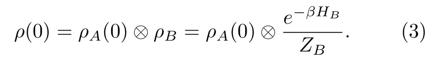
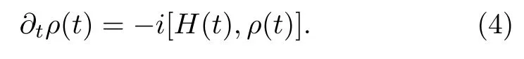
Here,ρA(0)andρBare the initial density matrix of system A and heat bath B,respectively.Because heat bath B is in a thermal equilibrium state at time 0,ρBhas a canonical form:βis the inverse temperature,1/kBT,andZB=TrB[e−βHB]is the partition function.Note that TrBis the trace taken over the heat bath.In the remainder of this paper,we always use the subscript to denote the degree of freedoms over which the trace is being taken.At a later timet,the density matrix of the composite system,ρ(t),satisfies the Liouville-von Neumann equation

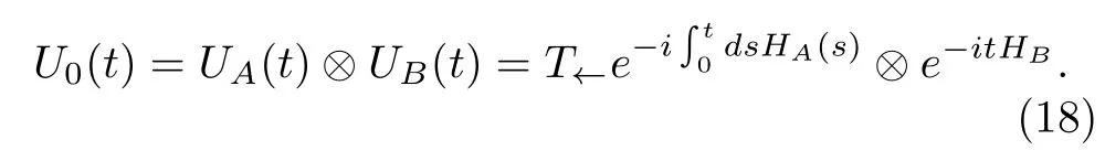
Planck’s constant ħ has been set equal to 1 here.If one could solve the equation,the dynamics of the open quantum system A is then obtained by taking the trace over the degree of freedom of the heat bath,i.e.,

Because this is a reduction procedure of the global density matrix,ρA(t)is also called the reduced density matrix of the reduced system A.

The solution of Eq.(4)can always be written formally as

by introducing the time evolution operator of the composite system,

where the symbolT←denotes the chronological timeordering operator.Considering that the open system A and heat bath B are initially uncorrelated,as in Eq.(3),the reduced density matrix of system A at timetcan also be expressed using a dynamical mapM(t):

where

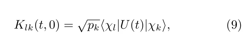
is called the Kraus operator.To obtain Eq.(8),we have used a spectral decomposition of the density matrix of the heat bath:

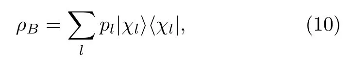
whereχland|χl〉are the eigenvalue and eigenvector of the HamiltonianHB,respectively,and

The dynamical mapM(t)has three important properties:convex linearity,trace preservation,and complete positivity[78,80,124].The dynamic map at arbitrary timet≥0 forms a one-parameter family{M(t)}.Although in principle this family describes the entire evolution of the open quantum system A,due to the complexity of the composite unitary evolutionU(t,0)for a generalH(t),it could be very involved.The simplest one-parameter family should be a Markovian family,namely,

Such a family is also called quantum dynamical semigroups[78,80,124].Importantly,one can alternatively express the dynamical semigroup using a linear differential equation or a MQME:

where the superoperatorLtis called the semigroup generator.Obviously,Eq.(12)is the quantum analogue to the Chapman-Kolmogorov equation in classical Markovian processes[125].In particular,for afiniteD-dimensional semigroup,the most general form of the generator was shown to be[80]

where the non-negative coefficientsra(t)are the eigenvalues ofA(t).Historically,Gorini,Kossakowski,and Sudarshan[77]were credited with establishing Eq.(14)for a time-homogenous quantum dynamic map,that is,M(t1,t2)depends only on the differencet2−t1.In this situation,the matrixAis time independent.Independently,also for the homogenous case,Lindblad[76]obtained Eq.(15)for the infinite-dimensional semigroups with bounded generators[124].In the literature,E-qs.(14)and(15)are called the Gorini-Kossakowski-Sudarshan-Lindblad(GKSL)equation.

B.Microscopic models

Eq.(14),and its equivalent Eq.(15),is only formally exact;its derivation does not depend on the concrete physical models.From the viewpoint of physics,it shall be more desirable if we could derive it fromfirst principles,e.g.,the microscopic expressions forFkandγab(t).Indeed,under the weak-coupling assumption,that is,the interaction termVin Eq.(1)is so weak that the influence of the open quantum system A on the heat bath B is small,and under several other key approximations,including the Born-Makovian approximation and the rotating wave approximation,one can indeed obtain a variety of MQMEs having the form of Eq.(14).In this paper,we will discuss four types of equations.Thefirst type is the time-homegeneous MQMEs[75,77,80,126],which we occasionally call the standard master equations in this paper.These equations have mainly been applied to issues related to how a system relaxes into a thermal equilibrium state[78,79]or arrives at nonequilibrium steady state[2,4,31,74,93,127]. The second type has time-dependent coherent dynamics,but the dissipator is static[14,16,18,128].These equations have often been used in quantum optics[78,96,98],e.g.,a twolevel atom interacting with a radiationfield while being driven by a classical time-varying electricfield[110].Their physical validity is ensured if the external driving field is so weak that its effect on the environment is negligible.The equations of the last two types fully depend on time,including the adiabatically(slowly)driven[10,17,20,83,84,129]and periodically driven MQME[24,25,102−105].Although the applicable regions of these four types of master equations are very distinct[124],all of them are very analogue to Eq.(14).In the remainder of this section,we will survey their derivations.

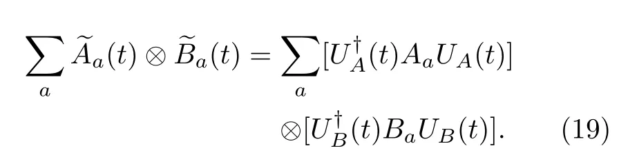
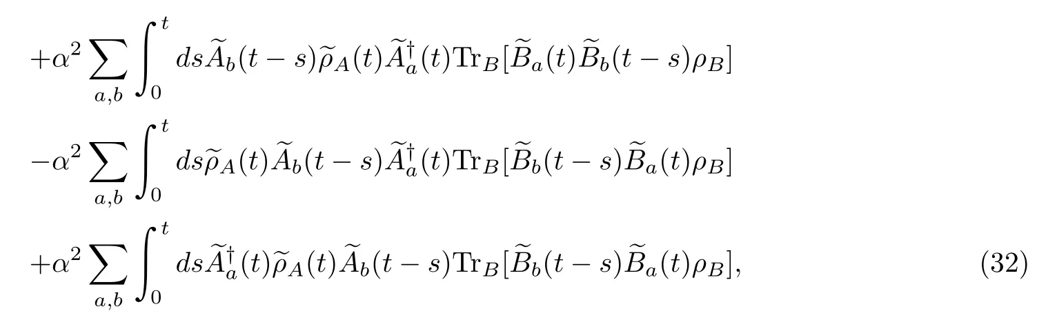
Wefirst write Eq.(4)in the interaction picture:

These notations with tildes indicate that they are inter-action picture operators with respect to the free Hamiltonians,namely,an arbitrary operatorO,

where the time evolution operator for the free Hamiltonians is

The explicit expression of the interaction picture operator for(t)is

According to the Nakajima-Zwanzig method[130,131],we introduce the projection operators

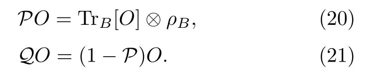
It is not difficult to prove that

Given the assumption TrB[BaρB]=0 and using the property(22),we applyPandQto Eq.(16)to obtain the following two equations:

The second equation has a formal solution:

Here,we have considered the vanishing initial condition,Q(0)=0,and have defined the propagator

Considering that the Liouville-von Neumann equation(4)is unitary,we may connectat two timessandt(s≤t)by

whereUV(t)=U0(t)†U(t)is the time evolution operator of the interaction picture operator(t),

and the symbolT→denotes the antichronological timeordering operator.Substituting Eqs.(25)and(27)into Eq.(23),we obtain

The reader is reminded that this result is a timeconvolutionless form with respect to:the density matrix on the right-hand side(RHS)depends on the timetinstead of the earlier times[78].

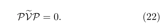
To simplify the complex integral in Eq.(29),we must resort to several approximations.Let us redefineVasαV,whereαis a small perturbation parameter.We expand the above equation up to the second order ofαand then arrive at

Here,we have performed a change of variables,s→t−s,and used an approximation

Inserting the concrete formulas of the projector operatorPandinto Eq.(30),we obtain

1.Static Hamiltonian

This is the standard case and is also the simplest case in which the Hamiltonian of the quantum system is time independent[77,126].The time evolution operator of system A is

where|εn〉andεnare the discrete energy eigenvector and eigenvalue ofHA,respectively.Then,the interaction picture operatora(t)has the following spectrum decomposition[78]:

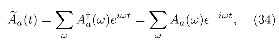
where

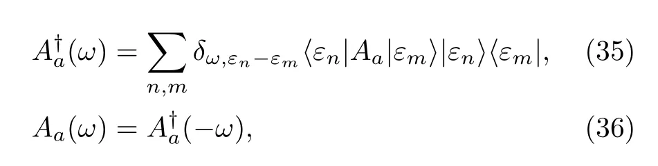
The energy differencesωare called Bohr frequencies,which may be positive or negative but always appear in pairs,andδis the Kronecker delta.These operators satisfy simple properties:

Therefore,Aa(ω)andare also called the eigenoperators ofHA.The reader is particularly reminded that different operatorsAa(ω)denoted by different indicesamay have the same frequencyω,as with the operatorsThis point is very relevant to the descriptions of QJT using either wave vectors or density matrices.Substituting the decomposition(34)into Eq.(32),we obtain

Here,we have used the time-homogeneous property of the two-time correlation function,

which is a result of the stationary heat bathρB.

There are two further approximations involved in the following derivations[78].Thefirst approximation is that the upper integral limittis replaced by+∞.This approximation is justified if the evolution time scaletof system A is far larger than the decay time of the heat bath.Specifically,significant non-zero contributions of these correlation functions in the integrals are arounds=0.Under this approximation,it shall be convenient to write these one-side Fourier integrals by the doubleside Fourier integrals,e.g.,

where

andP.V.denotes the Cauchy principal value of the integral.The other integrals can be rewritten analogously.Because the heat bath is at thermal equilibrium,these correlation functions satisfy the so-called Kubo-Martin-Schwinger(KMS)condition[132,133].In particular,this condition on the Fourier transform is

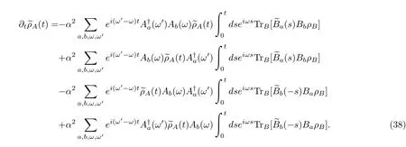
We will show later that this relation plays a key role in proving various FTs.The second approximation is the rotation wave approximation,or the secular approximation.Specifically,the terms with differentωandω′on the RHS of Eq.(38)are neglected.This approximation would be valid if a typical value ofω′−ωis far larger than the reciprocal of time,t−1.Given these two key approximations,doing a simple algebraic manipulation,wefinally obtain

where the Lamb-shift term is

Here,we have reabsorbed the small parameterαinto the interaction HamiltonianV.Note that these two approximations can be rigorously justified by taking the weak coupling limit,α →0,t→∞,and keepingα2tconstant[75,77,80,124].

Eq.(44)can betransformed back intothe Schr¨odinger picture.First,we know that

Because of

we immediatelyfind that the second term on the RHS of Eq.(46)is exactly the same as the RHS of Eq.(44)except that allA(t)therein are replaced byρA(t).After the above discussion,we have an conclusion that,if the decomposition(34)is true,the following equations,(38)-(45),would be available. This observation will guide our discussion about the time-dependent MQMEs.

2.Weakly driven Hamiltonian

Thefirst time-dependent case is the weakly driven Hamiltonian,

whereH0is the constant Hamiltonian of the bare system,H1(t)represents the coupling term of the bare system and some time-varying external force orfields,and the parameterγaccounts for the coupling strength.We assume thatγis of the same order of magnitude asαin the interaction HamiltonianV.This is the precise meaning of being weakly driven.Under this assumption,the time evolution operator of system A is approximated to be

When we substitute Eq.(49)into Eq.(32),the higher orders should beO(α2γ).Because we only retain the terms up to second order and neglect the other higher order terms,we re-obtain Eq.(44).However,we shall bear in mind that the decomposition,Eq.(34),is with respect to the eigenvectors and eigenvalues of the bare Hamiltonian,H0.Additionally,when we transform the time evolution equation into the Schr¨odinger picture,γH1(t)will be recovered because this Hamiltonian has a contribution to first order inγ.

3.Periodically driven Hamiltonian

It will be more desirable if we have a decomposition of Eq.(34)even if the Hamiltonian of the quantum system A is strongly driven. This is indeed possible ifHA(t)is periodic with a frequencyΩ [24,25,85,102−105,134−136],namely,

In this case,the famous Floquet theorem can be applied[137−139]:

where these time-independentϵnare called quasienergies,and the Floquet basis satisfies

The Floquet basis is periodic,that is,

It is not difficult to find that the solution

is still in the Floquet basis but with a shifted quasienergy

whereqis an arbitrary integer.Therefore,for the periodic Hamiltonian,the Floquet bases connected by E-q.(54)are equivalent in physics.We may project them into one Brillouin zone of width Ω.Using Eq.(51),we may see thata(t)still has a decomposition similar to Eq.(34)[140]:

or the Fourier coefficient with frequencyqΩ.Notice that in contrast to the static Hamiltonian case,the Bohr frequencyωhere depends on the external periodicity Ω.Substituting the new decomposition into Eq.(32),applying the same approximations as those in the static Hamiltonian case,and going back to the Schr¨odinger picture,wefinally obtain

where the Lamb shift is now

In this derivation,we have used the formula[140]

Compared with the evolution equation for the static Hamiltonian case,Eq.(46),the time dependence in E-q.(59)is through the operatorsAa(ω,t)andin addition to the time-dependent coherent dynamics.Nevertheless,the coefficientsrab(ω)remain static.

4.Adiabatically driven Hamiltonian

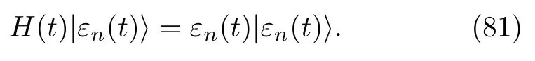
If the Hamiltonian varies in time very slowly,the adiabatical approximation can be applied to the operatorsk(t)[83,84,129,141].In this case,the time evolution operator of system A is

where|εn(t)〉andεn(t)are the instantaneous energy eigenvector and eigenvalues ofHA(t),respectively,and the phase in the exponential function is

With the above approximation,we have the following decomposition:

Note that there still exist two identities analogous to Eq.(37):

whereAa,mn(t)is brief notation ofAa,mn(t,t)and the Bohr frequency is

Different from previous cases,these frequencies are generally time dependent.For notational simplicity,we suppose that bothµmn(t)andωmn(t)are uniquely determined by the quantum numbers(m,n).The decomposition(64)remains inadequate;we still need another key approximation:

Under this approximation,we have the following decomposition:

The approximation(70)shall be justified ifHA(t)is almost unchanged in the time interval(t−s,t).Obviously,s～0 is preferred.Importantly,because of the very short decay time of these two-time correlation functions in Eq.(32),this condition is always fulfilled.We may relax the seemly strict condition ofs～0.To ensure the validity of the adiabatical approximation,Eq.(62),the durationtfof the non-equilibrium process shall be sufficiently large[142].In this situation,the change in the HamiltonianHA(t)would be very slow.Hence,in the interval(t−s,t)with nonzeros,the Hamiltonian could still be reasonably thought to be a constant operator.In particular,we expect that in the quantum adiabatic limit,ortf→∞,smay be anyfinite value.

Inserting Eqs.(64)and(71)into Eq.(32)and repeating the previous derivations,we obtain

where the Lamb-shift term is

Considering that

Distinct from the three previous cases,the coefficientsrabin the current case generally vary with time through the time-dependent Bohr frequencies,ωmn(t).Finally,we want to emphasize that Eq.(76)can be proved to be rigorous if one considers the weak coupling limit and quantum adiabatic limit simultaneously[83,143,144].

After a survey of the above derivations of these four types of MQMEs,wefind that all of them can be unified into a general formula:

where

and the positive and negative Bohr frequencies appear in pairs.Obviously,this formula follows the structure of Eq.(14).We can write its solution formally as

The whole exponential term,orG(t,0),is called the superpropagator of Eq.(77),or the dynamical map;see Eq.(8).

III.WORK IN CLOSED QUANTUM SYSTEMS

Let us start with the stochastic work of closed quantum systems.This concept is relatively simple and is also the foundation of studying the stochastic heat and work in open quantum systems.For convenience,throughout this paper,we suppose that the time dependence of the Hamiltonian of the quantum system A is always realized by a protocol,λ(t),namely,

as is the case for the time dependence of the instantaneous energy eigenvectors and eigenvalues of the Hamiltonian,

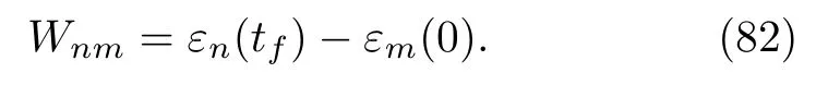
Because there is only one quantum system,we do not explicitly write the subscript A here.Consider that the non-equilibrium process of a closed quantum system is performed within the time interval(0,tf).According to the TME scheme[65,66],the stochastic work done by some external agents on the quantum system is defined as the difference in the instantaneous energy eigenvalues between the end and beginning of the process:

Following the terms named by Jarzynski[114],we call Eq.(82)the inclusive work.The reason for this will be given shortly.By repeating this process many times,we can construct the probability distribution of the work as

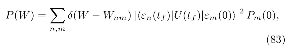
whereU(t)is the time evolution operator of the system andPm(0)is the probability offinding the system at the eigenvector|εm(0)〉at time 0.Because of the involvement of the Dirac function,Eq.(81)is not the most convenient form if we want to analyze the statistical properties of the work distribution.An alternative method is to resort to its Fourier transform or CF[4,54,55,69,71,117,125,145]:

Atfirst glance,both Eqs.(83)and(84)depend on the time evolution operator of the quantum system,U(t);no apparent advantages are shown in the latter expression.However,the CF can be rewritten as taking the trace over some operators,that is,

Note that the initial condition ofK(t,η)isρ0,and the symbolWη(t)is a superoperator;its action on an operator is a simple multiplication from the left-hand side(LHS)of the operator.In addition,we must emphasize that due to thefirst energy measurement,the density matrix,ρ0,may not necessarily be identical to the original initial density matrix of the system,ρ(0).This is an intrinsic difficulty of the work definition based on the TEM scheme[42,68].To avoid this additional complexity,throughout this paper,we assume that the initial density matrix of the system,ρ(0),is commutative withH(0).Then,ρ0=ρ(0).A typical example is the canonical density matrix,ρ(0)=e−βH(0)/Z(0),whereZ(0)is the partition function of the system at time 0 and is equal to Tr[e−βH(0)].

The work definition is not unique,for instance,if the Hamiltonian of the system is composed of two parts:

Following the terms in Eq.(48),we callH0the bare system.Because the coupling term,H1(t),is not required to be weak,the parameterγis absent here.A common physical model described by this Hamiltonian in textbooks is an electric dipole driven by a time-varying electricfield[146].Assuming thatH1(t)vanishes at time 0,we may alternatively define the work done on the bare system using the TEM scheme as

and its distribution is obtained by

where

We can easily prove that the operator0(tf,η)still satisfies the Liouville-von Neumann equation(4)with an initial conditione−iηH0ρ0,whileK0(t,η)satisfies a time-evolution equation given by

Its initial condition remainsρ0,andis a superoperator acting on operators on its LHS.

Let us give several comments on Eq.(87).First,if the parameterηis set to be zero,Eq.(87)is reduced to the Liouville-von Neumann equation(4),andK(t,η)is simply the density matrix of the system,ρ(t).Second,ifρ0is a thermal equilibrium state with inverse temperatureβ,Eq.(87)withη=iβhas a simple solution:

According to the probability interpretation of the CF,Eq.(84),we proved the quantum JE in the closed quantum system.On the other hand,this thermal equilibrium condition also indicates that(0,iβ)is proportional to an identity operator.Hence,the Liouvillevon Neumann equation of(t,iβ)has a trivial solution,(t,iβ)=1/Z(0).Using the second equation in Eq.(85),we are led to the JE again.Of course,the most straightforward proof of this equality is to apply the first equation in Eq.(85)and setη=iβtherein.Very analogous results can be obtained in Eq.(93),

and the quantum Bochkov-Kuzovlev equality(BKE)[50,115,147]is proved in this case.These formulas were previously found by us,but the backward-time versions of Eqs.(87)and(93)were utilized therein[11,16]. Third,Eq.(87)can be regarded as the quantum version of the time evolution equation about the CF of the classical inclusive work[88,116,117,148].According to the quantum-classical correspondence principle[146],as Planck’s constant ħ tends to zero,the commutator is reduced to the Poisson bracket,and operators are replaced by ordinary functions[149].Hence,the classical correspondence of Eq.(87)is

wherezrepresents the phase coordinates of the closed classical system and{,}PBdenotes the Poisson bracket. It is not difficult to prove that the integral of the functionK(z,t,η)is simply the CF of the classical work[114].On the other hand,based on the celebrated Feynman-Kac(FK)formula[150],Eq.(96)has a path integral representation.Because of this,we called Eq.(87)the quantum FK formula[11,16].Analogous results are also true for the exclusive work case.A further explanation is presented in Appendix A.Finally,in addition to the straightforward definition ofK(t,η),Eq.(85),the time evolution equation(87)also reminds us that it has an alternative expression using the Dyson series[151]:

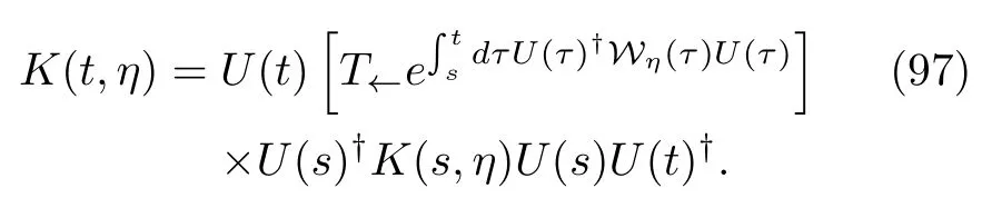
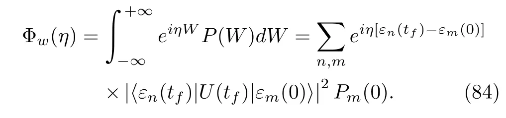
FIG.1 Inset:the quantum piston model.At time 0,the position of the moving wall is λ(0).The system is in thermal equilibrium with a heat bath whose inverse temperature iswhere ε1is the first energy level of the infinite square-well potential,which equals ħ2π2/2mλ(0)2.The system is then disengaged from the heat bath,and the wall moves at a uniform speed up to a new position,λ(tf)=2λ(0).The left and right columns are the probability distributions of the inclusive work(in units of ϵ1)and their corresponding CFs at two moving speeds:the speed of the left column is v=0.1 ε1λ(0)/ħ,while that of the right column is v=10.0 ε1λ(0)/ħ.The black solid and dashed lines in the lower panels are the real and imaginary parts of these CFs,respectively.They are calculated by directly applying Fourier transforms to the work distributions in the upper panels.The circle and star symbols are the real and imaginary parts of the CFs obtained by solving the time evolution equation(87).The red solid and dashed lines are the real and imaginary parts of the CFs obtained by solving(4)with an initial condition e−iηH(0)ρ0.Because these red lines are exactly overlapped with the black lines,we obviously cannot read them.For convenience,we have let ħ =1, ε1=1,and λ(0)=1 in the computations.

This formula connects two WCOs at two time points,sandt,wheres≤t.We may re-express the above equation by exchanging the positions ofK(s,η)andK(t,η)and obtain

This mimics Eq.(27).The primary advantage of using this seemly complex expression forK(t,η)is that we may approximate it by expanding the time-ordered exponential term in terms ofWη.We will show its applications in the next section.

To illustrate the application of Eq.(87),we concretely calculate the CF of a quantum piston with a moving wall[152];see the inset of Fig.(1).Suppose that the uniform speed of the wall isv.We are interested in this model because the piston Hamiltonian appears to depend only on the kinetic energy,p2/2m.Because the superoperatorWηis always zero,Eq.(87)seems problematic in calculating the CF of the inclusive work.However,this is not the whole story:the Hamiltonian acts on the Hilbert space of the system of the quantum piston,and the space is changing in time due to the moving wall;therefore,H(t)indeed depends on time.This point would become clear if we explicitly wrote and solved this equation in the instantaneous energy representation.Figure(1)shows two probability distributions of the inclusive work at two moving speeds and their corresponding CFs.These distributions are directly calculated using the definition,Eq.(83).The CFs are obtained in two ways:performing Fourier transforms of these work distributions(see the black solid and dashed lines)or solving Eq.(87)by a simple mathematical program and then utilizing Eq.(85)(see the symbols in the samefigure).We have assumed that at time 0,the piston is in a thermal equilibrium state.We see that at a low pulling speed,the results obtained under these two different methods are in good agreement,but an apparent deviation has occurred at the higher speed.We think that this discrepancy is induced by the numerical errors in solving the differential equation(4);Wη(t)is a rapidly oscillating term with respect to time in the energy representation.To avoid additional numerical efforts,wefind that solving the Liouville-von Neumann equation(4)of(t,η)with an initial conditione−iηH0ρ0is a simple and effi-cient method.The calculated results are shown in the same panels using the red solid and dashed lines.Wefind that they are highly consistent with those obtained by directly performing Fourier transforms of the work distributions.

IV.HEAT AND WORK IN OPEN QUANTUM SYSTEMS

A.TEM scheme applied to the composite system

As we have mentioned in Sec.(II),an open quantum system A and its heat bath B can be combined as a closed composite system.Hence,the TEM scheme can be naturally extended to define stochastic thermodynamic quantities in the open situation.The global Hamiltonian is given by Eq.(1).Note that we have assumed that its time dependence is through a protocolλ(t)acting only on the quantum system A.

We are concerned about the changes in energy of subsystem A and heat bath B.Following Kurchan[65],Talkner et al.[8]and Esposito et al.[4],we define the difference of the energy eigenvalues of the heat bath Hamiltonian,HB,between the end and beginning of the non-equilibrium process as the heat released by quantum system A.Formally,the stochastic heat is

Hence,its probability distribution is

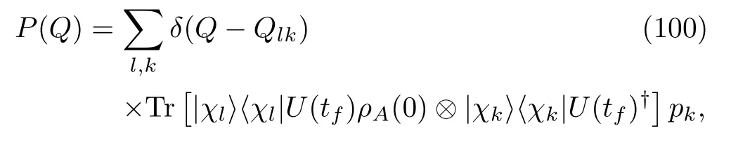
FIG.2 A schematic diagram describing the work definition(102)based on the TEM scheme applied to the combined quantum system(the blue circles)and heat bath(red squares).The evolution of the global system is unitary under the Hamiltonian in Eq.(1).The green arrow on the right-hand side denotes the projected energy measurement on the system and bath at the end time tf.

wherepkis the probability offinding the bath at the eigenvector|χk〉;see Eqs.(10)and(11).Correspondingly,the Fourier transform of the distribution or the CF of the heat is

The reader is reminded that we did not impose any restriction on the initial density matrix of the open system A.

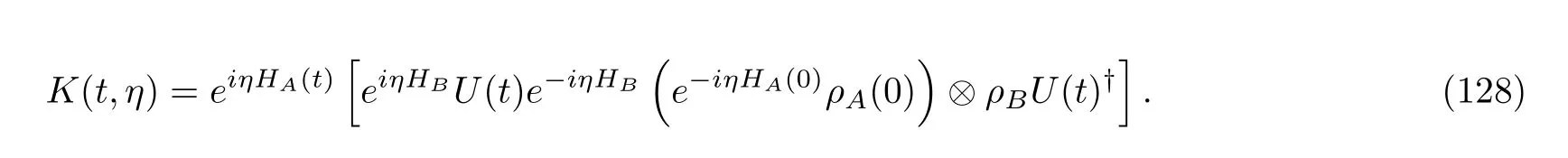
Considering that the global quantum system(1)is closed,we may define the inclusive or exclusive work as we did in the preceding section.In particular,considering that the interaction between system A and heat bath B is very weak,we can approximate the inclusive work as[8,101]

by disregarding the effect of the interaction term.Here,εm(t)is the instantaneous energy eigenvalue ofHA(t).

To ensure the validity of the work definition,we have to impose the condition

Therefore,in terms of the condition of the initial density matrix,the case of work is distinct from the case of heat.Given these notations,we may easily obtain the distribution of the inclusive work of the open quantum system:

wherePkm(0)is the joint probability offinding the composite system at a state|εm(0)〉⊗|χl〉,

Note thatρ(0)is assumed to be uncorrelated;see E-q.(3).Correspondingly,we may write the CF of the inclusive work of the open quantum system as

According to the work terms proposed by Jarzynski[114],if the Hamiltonian of quantum system A is composed of two parts,as in Eq.(88),i.e.,

we can define the exclusive work and its CF as E-qs.(102)-(106)with slight modifications.For instance,if we remove the timetfand the circle brackets on both sides on the RHS of Eq.(102),this equation is simply the formal definition of the exclusive work,

We may apply similar treatments to the other equations,and thus,we do not write them out explicitly.An important observation is that although the heat and work are different in energy transfer forms,both of their CF-s have mathematical formulas analogous to Eq.(85).

Hence,we are able to introduce HCO and WCO and derive their time evolution equations.Finally,we want to mention that we may also define the stochastic inner energy of system A and its CF.The interested reader may realize this straightforwardly.

B.Heat characteristic operator

According to the structure of Eq.(101),we call the whole term in its trace the HCO of the quantum open system A,i.e.,

This newly defined operator satisfies a simple time evolution equation,

and its initial condition isρA(0)⊗ρB.We see that there are similarities between Eqs.(110)and(93).Although the above equation is exact,it is inconvenient because of the involvement of the complicated global evolution.The idea of QMEs may be used to address this issue[78].To our knowledge,Esposito et al.[4,153]were thefirst to carry out such an effort.Because they used a modified Hamiltonian,they derived an evolution equation that is distinct from our equation.

Following the work in Sec.(II.B),wefirst write Eq.(110)in the interaction picture with respect to the free Hamiltonian,HA(t)+HB:

Based on the projection operators defined in Eq.(20),it is not difficult to prove that

Applying this property and applyingPandQto Eq.(111),we obtain

The second equation has the formal solution

where we have considered the conditionand defined the propagator

On the other hand,the similarity between Eqs.(111)and(87)reminds us thatat two time pointssandt(s≤t)are connected by

whereUV(t)=U0(t)†U(t)is the time evolution operator of the interaction picture operator(t);see Eq.(28).Substituting Eqs.(115)and(117)into E-q.(113),we obtain

The reader is reminded that this equation also has a time-convolutionless form that is analogous to Eq.(29).

To eliminate the complex integral in Eq.(118),we must resort to some approximations,as we did in deriving MQMEs previously.First,redefiningVasαV,we expand the above equation up to second order inαand then obtain

This approximation is based on

where we made the change of variabless→t−s.To explicitly write the projector operatorP,the superoperatorshand,we obtain

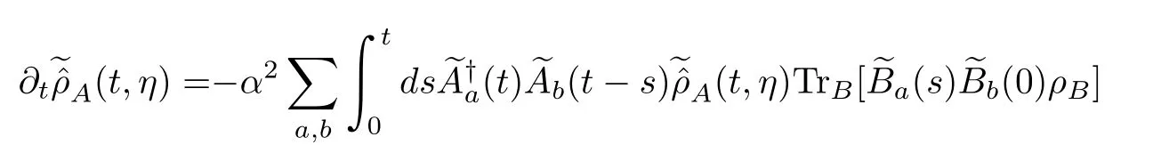
where

and its initial condition isρA(0).Because taking the trace of the operatorA(t,η)(the interaction picture operator)over the degree of freedom of system A is just the CF(101),we also call it the HCO of the open quantum system A.The next step is to check whether Eq.(121)has a Markovian form with respect to concrete open quantum systems.We have to do this on a case-by-case basis.

1.Static Hamiltonian

Inserting the decomposition(34)into Eq.(121),we obtain

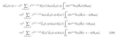
According to the procedure for deriving the MQEMs,what follows is to apply the two approximations.The rotation wave approximation seems to still be reasonable.However,the replacement of the upper integral limittby an infinity or the Markovian approximation given by Esposito et al.[4]seems to be problematic here.As we have mentioned before,the validity of the replacement is based on the fact that the signifi-cant non-zero contribution of the two-time-correlation functions,the trace terms TrBin Eq.(123),shall be arounds=0[78,80].Obviously,the presence ofηhere changes the situation.For instance,if we chooseηto be far larger than the timet,the second integral in the equation is negligible.In contrast,the same integral but with an upper limit of infinity is not at all zero.However,we must emphasize that this approximation will become exact in the weak-coupling limit,namely,α→0,t→∞and keepingα2tconstant[75,77,80,124].For a physically relevant finiteα,the Markovian approximation should work well for the cases in whichηis approximately 0 or the timetis very large;for other cases,it is at most considered as an ansatz to obtain a simple Markovian evolution equation.Note that the validity of the MQMEs shall be understood in the same manner[80].Therefore,if we admit these two approximations,introduce the double-sided Fourier integrals(some details are presented in Appendix B),and perform a simple calculation,we obtain the following result:

Eq.(124)can be transformed back into the Schr¨odinger picture by applying a procedure analogous to Eq.(46).

2.Weakly driven Hamiltonian

This case is almost the same as the static Hamiltonian case.We may obtain Eqs.(123)and(124)again except that the Bohr frequency,ω,and the spectral decomposition,Ab(ω)andA†a(ω),are all with respect to the bare HamiltonianH0;see Eq.(48).

3.Periodically driven Hamiltonian

Because the spectral decomposition,Eq.(56),is exactly the same as that of the case of the static Hamiltonian,we obtain a time evolution equation analogous to Eq.(59)under the two approximations in the Schr¨odinger picture;the only difference is that an additional exponential phase factor,eiηω,is present in front of the first operatorAb(ω,t)here.To our knowledge,Gasparinetti et al.[24]was thefirst to obtain such a time evolution equation.Rather than the very general form that we obtained here,they were concerned with a specific two-level system and wrote it in the Floquet basis representation.

4.Adiabatically driven Hamiltonian

Compared to the previous three cases,the adiabatically driven situation is slightly complicated because the presence ofηin Eq.(121)seems to render the approximation in Eq.(70)invalid in general:the correlation function is significantly non-zero arounds=η,whereasηis arbitrary,andsdoes not need to be a small number.However,this difficulty will disappear if we take the weak coupling limit and the quantum adiabatical limit simultaneously[83,143,144].We have given an explanation in Sec.(II.B.4).Hence,we can obtain a time evolution equation analogous to Eq.(76)except for the presence of the factoreiηωmn(t)in front of thefirstAb,mn(t).

Based on the above discussions,wefind that for the four types of QMEs that we have studied so far,their evolution equations of the HCO can be unified as specific cases of the generic case:

We may write the solution of Eq.(125)formally as

where the whole time-ordered exponential term is a su-perpropagator.The CF of the heat is then

We must bear in mind that Eq.(125)has a rigorous meaning only in the weak coupling limit and quantum adiabatical limit(only for the adiabatically driven case).Otherwise,it shall be regarded as an approximation in solving the HCO of the open quantum system.

We expect that this equation shall be sound under the conditions of smallerηand largert.

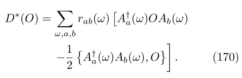
C.Work characteristic operators

There are two equivalent methods for obtaining the CF(106)of the inclusive work.Wefirst call the whole term in its trace the WCOK(t,η)of the open quantum system,namely,

Here,we added two square brackets.We immediatelyfind that the term in the brackets is almost the same as the HCO,Eq.(109),except that the initial“density matrix” of the system A has becomee−iηHA(0)ρA(0).We observed the same structure when we investigated the WCO in the closed quantum system;see the second equation in Eq.(85).This also explains why we called it the HCO in closed quantum systems even though there is no heat concept therein.Therefore,the CF of the inclusive work can be evaluated byfirst solving the time evolution Eq.(125)with the new initial condition and then taking the trace.This procedure is shown in the following equation:

This method has been used by Silaev et al.[18]and Cuetara et al.[25]in several special MQMEs.On the other hand,we are curious as to whether there exists a time evolution equation of the WCO that is defined only on the degree of freedom of system A similar to Eq.(125):when we solve it,we can obtain the CF of the inclusive work by simply taking the trace over the open quantum system A.This consideration is very natural because the roles of the work and heat are equal.This is not difficult to realize if we regard the whole term in the trace of Eq.(129)as the WCO,KA(t,η),of the open quantum system A.Taking the time derivative and using the known Eq.(125),we obtain

We must emphasize that the initial condition ofKA(t,η)is the genuine density matrix,ρA(0).When we solve the equation,the CF of the inclusive work is then

From the perspective of numerical calculations,the former method is more attractive than the latter.We see that these two methods are parallel to those that we used for the inclusive work in the closed quantum systems;see Eqs.(85)and(87).

In addition to the inclusive work,for the given Hamiltonian(107),we have defined the stochastic exclusive work,Eq.(108),of the open quantum system.Mimicking Eq.(128),we also define the WCO

Using very similar arguments,we can calculate the CF of the exclusive work by solving Eq.(125)with the initial conditione−iηH0ρA(0)and then taking the trace over the degree of freedom of system A,namely,

In addition,we can also define the whole term in the trace of the above equation as the WCO,K0A(t,η),on the open quantum system A.Then,we have an alternative method to obtain the CF by directly solving the following equation:

where

Note that its initial condition isρA(0).

These pretty results raise an interesting question:can we directly obtain Eqs.(130)or(134)using the idea of QMEs as we have done in the case of heat?We have mentioned that the roles of work and heat are equal.Hence,one should be able to obtain the time equations concerning the workfirst and then derive the equations for the heat later.To answer this question,we write the time evolution of the operator defined in Eq.(128):

We transform it into the interaction picture with respect to the free HamiltonianHA(t)+HB,

where

In analogy to Eq.(112),we prove

Hence,applying the projection operatorsPandQto Eq.(137)once more,we obtain

Considering the vanishing initial condition,Q(0,η)=0,we write the formal solution of the second equation as

where the superpropagator is

Substituting the solution into Eq.(141),we have

To obtain this result,we have used the following two approximations:

and

Combining Eqs.(145)and(146),explicitly writing the projection operatorP,the superoperatorswand,and performing a simple algebraic manipulation,we have

which can be easily seen from the two equivalent expressions ofK(t,η)in Eqs.(85)and(97),the RHS of Eq.(149)can be dramatically simplified into

We immediatelyfind that Eq.(152)is simply the RHS of Eq.(121)ifA(t)therein is changed toand if the whole formula is multiplied by the exponential phase factor,Therefore,after combining Eqs.(149)and(152)and applying the detailed process with respect to the concrete HamiltonianHA(t)as we did in the heat case,we arrive at the general Eq.(130)for the WCOs on these open quantum systems.A very analogous procedure can be applied to the case of the exclusive work as well.Because this is straightforward,we do not present it here.

Before concluding this section,let us give two comments on the general Eqs.(130)and(134).First,the valid conditions of these equations are exactly the same as those of Eq.(125).Second,for the adiabatically driven Hamiltonian,Eq.(130)has a concise form[17].According to Eq.(68),we can move the exponential term,e−iηHA(t)in Eq.(130),outside of the first bracket to cancel the front term,eiηHA(t),and find that the original equation is simplified to

We see that this structure is consistent with that of Eq.(87)for the inclusive work in closed quantum systems.On the other hand,Eq.(134)also has a simpler formula for the case of a weakly driven Hamiltonian[16].In this situation,considering

we can cancel the two exponential terms aboutH0in Eq.(134)and rewrite the original equation as

Intriguingly,this structure is consistent with that of Eq.(93)for the exclusive work in a closed quantum system.

D.Mean heat and work

Itisinteresting to compare the thermodynamicquantitiesdefined in ST tothosein EQT[47,81,82,84−87,105,136].We expect that the averaged stochastic quantities of the former would agree with those of the latter.According to the definitions of CF-s,Eqs.(101)and(106),the averages of the stochastic heat and work can be calculated by taking derivatives of these functions with respect toηatη=0,e.g.,the released average heat,

Alternatively,we can also obtain the same result by applying a Taylor series expansion of these CFs aboutη=0.For instance,wefirst rewrite Eq.(125)as

Note that the lowest order of the superoperatorQηofηis thefirst order.Based on the superpropagator,G(t,s)in Eq.(79),where time 0 is replaced by times(≤t),the solution of the above equation has an integral ex-pression:

Obviously,thefirst term on the RHS is the density matrix of the open quantum system A at timet,ρA(t).Substituting the solution into Eq.(127),using a Taylor series aboutη=0,and collecting all coefficients to first order inη,we formally obtain the average heat:

To obtain the second equation,we have used an important identity:

whereL∗(t)is the dual ofL(t)and is equal to

The dual superoperatorL∗(t)has the trivial property

whereIrepresents the identity matrix.

Applying the analogous arguments to Eqs.(129)and(132),wefind that the average inclusive and exclusive works are

respectively.Note that the second terms on the RHSes are the same because we have imposed the conditionH1(0)=0 in the case of the exclusive work.Obviously,the differences between the first two terms on the RHSes are the changes in the systems’mean inner energies within afinite time interval,(0,tf).Hence,Eqs.(163)and(164)are simply thefirst law of thermodynamics realized in the various MQMEs.

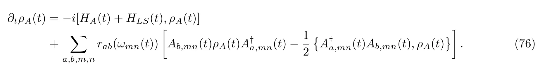
Let us check whether the above mean stochastic heat and work are the same as the definitions in the literature[47,84,86,105,136,155]. In adiabatically driven MQMEs,Alicki has split the change in the mean inner energy of the open quantum system A into two parts:

This formula is a simple integral expression for the time derivative of the mean inner energy within thefinite time interval,(0,tf),which can always be done for any MQME and is not essentially confined to the adiabatically driven case.Since Pusz and Woronowicz[155]interpreted thefirst term on the RHS as the work done by some external agent in theC∗-algebraic context,Alicki called the second integral the heat supplied to the system by its heat bath.The physical validity of the heat definition is supported by the second law of thermodynamics in adiabatically driven MQMEs.Alicki’s heat and work definitions were broadly applied in EQT[47].Superficially,Eq.(159)is very distinct from Eq.(165).However,when we insert the master equation(76)into Alicki’s heat definition,we find that

where we have used Eq.(68).The integral on the RHS is simply Eq.(159)in these particular MQMEs.Hence,the mean stochastic heat is indeed consistent with the heat proposed by Alicki.Because of the samefirst law of thermodynamics,the mean stochastic work is also equivalent to the work definition in Eq.(165).Interestingly,this also reminds us that,in the adiabatically driven case,the mean stochastic work has an integral expression.Even so,we must emphasize that we cannot generalize these observations to the other types of MQMEs,that is,in general,

An obvious example is periodically driven MQMEs[105,118,136]. Thisfinding is not very surprising.After all,the splitting of the LHS in Eq.(165)is not unique in mathematics. Hence,there is no prior reason to treat these two terms precisely as the physical heat and heat.In contrast,Eq.(159)is a measurement-based heat definition.

It is interesting to see that Eq.(164)is consistent with other work definitions that are restricted to weakly driven MQMEs[17],where the Hamiltonian of the open quantum system A is Eq.(48).In the spirit of Alick,the change in the average energy of the bare Hamiltonian,H0,can also be split into two parts:

where the dual dissipator is

We can prove that for weakly driven MQMEs,based on Eq.(154),the second integral term in Eq.(169)is equal to

The RHS is simply Eq.(159)in these particular MQMEs.Hence,we alsofind that the mean stochastic exclusive work here has an integral expression;see thefirst integral in Eq.(169).As is the inclusive work case,these formulas are only valid for these specific MQMEs.Boukobza and Tannor[86]have independently proposed very similar heat and work definitions.They thought that their definitions were also applicable to other MQMEs.Because of the non-uniqueness of the splitting of Eq.(169),this statement shall be treated carefully.Finally,we want to note that,in periodically driven MQMEs,Eq.(159)is also consistent with the heat definitions proposed by Langemeyer and Holthaus[136]and Szczygielski et al.[105].We have illustrated this concretely in a two-level system[119].The interested reader is referred to our paper.

V.FLUCTUATION THEOREMS

As we mentioned in Sec.(I),one of the primary motivations of studying stochastic heat and work is to explore the validity of a variety of FTs in the quantum regime.In the classical situation,based on a theorem about average quantity or about the probability distribution of a stochastic thermodynamic quantity,we roughly divide these theorems into integral or detailed FT correspondingly.For instance,the JE belongs to the former,while Crooks’equality is an example of the latter.In this section,we also utilize these terms.Although a detailed FT can result in an integral FT,the proof of the latter is usually relatively easy because we do not need to resort to the time-reversal concept.In addition,the reader will see that the conditions of these two types of FTs are slightly different due to the involvement of quantum measurements.

A.Integral FTs

These theorems are implied in the mathematical structure of Eq.(125).Because the heat bath is in thermal equilibrium,the KMS condition on the Fourier transforms,Eq.(43),reminds us that the action of the superpropagatorˇL(t,iβ)in Eq.(125)on the identity operatorIis exactly zero,

This almost trivial property can account for several integralfluctuation theorems.The first theorem is about the stochastic heat(99).According to Eq.(127)and the meaning of CF,we immediatelyfind that

where we have used the subscriptcto denote that the equality is valid for a completely random initial density matrix,which is denoted byC,e.g.,in aD-level quantum open system,C=I/D.

Eq.(172)also accounts for the remarkable equalities about the exclusive and inclusive work.According to Eq.(129),if the system’s initial density matrixρA(0)is the thermal equilibrium state with the heat bath inverse temperatureβ,we must have

where the subscriptthdenotes the initial thermal state andZ(t)is the equilibrium partition function,withZ(t)=Tr[e−βHA(t)].This theorem is simply the quantum JE in the general MQME.We can verify this intriguing result by solving the time evolution equation(130).Becauseη=iβ,we easily see that it has a simple solution:

Taking the trace over the degree of freedom of the quantum system A,we re-obtain the JE of the inclusive work.Very analogous results can be derived for the exclusive work,Eq.(108):

This is called the quantum BKE[16]in the general MQME,Eq.(77).Analogously,givenη=iβ,the solution of Eq.(134)is simply

The validity of the quantum JE is not trivial.We know that in the classical regime,the JE is always accompanied by a condition that the open classical system has an instantaneous thermal state solution[89,114].This condition was also equivalent to the instantaneous detailed balance condition.Physically,this condition indicates that if the external protocol isfixed at a specific value,the system will relax to the thermal equilibrium state under thisfixed protocol.If we extend this observation into the quantum regime,we might expect that only if the generator of Eq.(77)satisfies

would the quantum JE be valid.Indeed,for closed quantum systems and the adiabatically driven Hamiltonian case that we discussed before,this connection was well established[7,10,11,17].However,the scope of validity of Eq.(174)is beyond this condition.For instance,there is noρth(t)in periodically driven MQMEs[105,124,135]or in weakly driven MQMEs.Therefore,our proof shows that the most fundamental aspect ensuring the validity of thesefinite-time FTs is the KMS condition,Eq.(43).It has been known for a long time that the KMS condition and the detailed balance condition have a deep connection in a time-homogenous dynamical semigroup possessing a stationary state[81,156−158].This connection is broken in the general time-dependent MQME,but the KMS condition remains because the heat bath is still in thermal equilibrium.Intriguingly,Spohn and Lebowitz[81]noticed that the KMS condition was also essential for deriving some basic postulates of the thermodynamics of irreversible processes,e.g.,the Onsager relations and the principle of minimal entropy production.They particularly noted that“To state it(the KMS condition denoted by us)in a somewhat oversimplified way:In our model irreversible thermodynamics follows from the fact that the reservoirs are at thermal equilibrium”.The irreversible behaviors described by Eq.(77)of course occur for the same reason.Our conclusion also agrees with that drawn by Talker et al.[8].They proved that the JE is always true for very general open quantum systems with arbitrary time-dependent protocols,as long as the interaction between the quantum system and the heat bath is sufficiently weak.Contrary to our formulas,their results did not rely on Markovian or rotation wave approximations.The weak interaction condition amounts to the condition that the heat bath is always in a thermal state and is unperturbed by the open quantum system.

B.Detailed FTs

In classical stochastic systems,the integral FTs can always be traced to their detailed versions concerning the probability distributions of the stochastic thermodynamic quantities of forward and backward processes.Indeed,Talkner et al.[4,8,69,71]showed that this is also true in closed quantum systems.In particular,they expressed the results using the symmetric property of CFs.In this section,for general MQMEs,Eq.(77),we present the detailed versions for the integral FTs,Eqs.(173),(174),and(176).To this end,we need to define the backward non-equilibrium quantum process.We call a process forward if the protocol driving system A isλ(t),whereas a process is backward if the same quantum system is driven by a time-reversed protocol,

wheret+s=tf.To distinguish the backward process from the forward process,we specifically use the symbols with overlines to represent the physical quantities of the backward process.We also use the notationsto denote the time of the backward process.In addition,we further suppose that the Hamiltonian of the global system is time-reversal invariant(TRI).Specifically,the Hamiltonian of the composite system A and heat bath B of the backward process is

where the time-reversed Hamiltonian of system A,of the heat bath and of the interaction are

respectively,and Θ is the time reversal operator[142].The last equation in Eq.(181)is true because the time dependence of this Hamiltonian is realized only through the external protocolλ(t).According to Eq.(2),the TRI interaction HamiltonianVindicates that the timereversal types of the operatorsAaandBamust be consistent with each other.Specifically,if

whereδais equal to+1 or−1 depending on the timereversal type ofAabeing even or odd.Comparing E-q.(180)with Eq.(1),we can see that the dynamics of the backward process is the same as that of the forward process except that the protocol is changed into the new process,(s).Therefore,the CF of the heat of the backward process is

We do not specify the uncorrelated initial condition of the backward process yet.This general equation does not provide us the explicit expressions ofandor their concrete connections with those quantities of the forward process;we have to obtain them by investigating concrete Hamiltonian systems.Note that we did not add an overline overrabbecauseVis TRI.

Given the above notations,we are in a position to discuss the relation between the CFs of the forward and backward processes.Let us start with the case of heat.According to the formal solution,Eq.(126),we write Eq.(127)with a completely random initial density matrix as

The second equation results from the fact thatCis proportional to the identity matrix and the dual definition

where

In the third equation,we applied an identity for the time reversal operator Θ[142]:

The last equation is obvious if one writes the timeordered exponential term explicitly.Now,we want to show that the whole term in the trace of the last equation is the formal solution of Eq.(186)but with=iβ−ηat timetf,that is,

We again emphasizes+t=tf.To prove this conjecture,we temporally denote the whole term on the RHS of Eq.(191)Taking its derivative with respect to times,we obtain

It is worth noting that the condition of the TRI interaction HamiltonianVimplies that the Fourier transforms of the two-time correlation functions,Eq.(41),satisfy

This relation also indicates that the matrix{rab(ω)}is not only Hermitian[78]but also composed of real or purely imaginary numbers.A brief explanation of Eq(193)is presented in Appendix D.Therefore,if E-q.(192)is really equivalent to Eq.(186),we need to check the following two equations:

In Appendix C,we will show that Eqs.(194)and(195)are exactly true for all the MQMEs that we discussed so far.In the general situations,we can simply regard a process as backward if itsand Bohr frequencyωare defined by the above two equations.

Substituting Eq.(193)and these two identities into Eq.(192),and noticing the KMS condition,Eq.(43),wefind that

where its initial condition isC.Comparing the time evolution equation with Eq.(186),we conclude that Eq.(191)is indeed true.Therefore,we can continue Eq.(187)and obtain

According to the relation between the CF and probability distributions,e.g.,Eq.(84),we have

What we have done can be generalized to the cases concerning the inclusive and exclusive work.In the former,according to Eq.(129),we have

Based on the previous discussion,in the last equation,the whole term except for thefirst exponential operator is simply the solution of the backward equation(186)with=iβ−η.In particular,here,its initial condition is

Hence,the whole term,including the termis simply the WCO of the inclusive work of the backward process;see the definition in Eq.(129).Therefore,

If we represent this relation using probability distributions,we obtain the remarkable Crooks’equality about the inclusive work:

where the free energy difference isβ∆F=lnZ(tf)−lnZ(0).In the exclusive work case,we can utilize a very analogous discussion and ultimately obtain

Note that in this equality,the initial condition of the backward process must be the thermal statee−βH0/Tr[e−βH0].On the other hand,to ensure that the work definition based on the TMS scheme is reasonable,we also require that the initial density matrix is commutative with the Hamiltonian of the system at the initial time.This requirement is essential in both the forward and backward processes.Hence,in this case,Eq.(203)additionally imposes a condition thatH1(t)must be zero at both the beginning and end time.Interestingly,this condition is absent in the quantum BKE,Eq.(176).In classical stochastic processes,this condition is not needed either.Finally,let us conclude this section by noting that,if we integrate these detailed FTs,Eqs.(198),(202),and(204),with respect to the stochastic heat and work,we will again obtain the previous integral FTs.

VI.QUANTUM JUMP TRAJECTORY

The density matrix and MQMEs are essentially an ensemble description of open quantum systems.Nevertheless,in practice,one usually addresses individual quantum systems.This situation is very similar to classical Brownian motion:we can mathematically describe the evolution of an ensemble of Brownian particles using probability distributions and the Fokker-Planck equation[125,145],but in real experiments,e.g.,single-molecule experiments[159],one often measures the motion of individual Brownian particles,and the equation describing the motion is the Langevin equation.Therefore,we may naturally ask whether there are formulas that can describe the dynamics of single open quantum systems.The QJT was shown to be one such formula[78,97,98].The idea behind the QJT started in the sixties and was intimately connected with theoretical efforts on fully quantum mechanical treatments of photon counting experiments in quantum optics,where a detector monitors a quantum system over a time interval and records the arrival times of the photons[91,94,99,110,111,121,160−162].This concept became increasingly important after observing or manipulating single quantum system became possible[163−172].In the developing history,the QJT has been given different names,e.g.,the Monte-Carlo wave function method[173],the stochastic wave-function method[78],the unravelling of the quantum master equations,and quantum trajectories[96].We refer the reader interested in the historic overview of QJTs to the review papers[95]or the relevant monographs[78,96,97,174].Although it was known very early that the QJT can be used to re-obtain all the results given by MQMEs[78]and that the latter are very fundamental in investigating irreversible thermodynamics[81],its potential applications in thermodynamics were almost completely unrecognized for almost four decades1An exception might be the entropy production study conducted by Breuer[100]..In this section,we give a self-contained explanation about QJTs.Our discussion is based on basic quantum mechanics and simple probability knowledge and does not rely on other advanced contents,e.g.,quantum stochastic calculus[176].In particular,we attempt to present our theory under the framework of the TEM scheme.In previous studies,this energetic perspective of the origin of QJTs was usually introduced directly without explicit explanation.We think that this might be an obstruction hindering the appreciation of the values of QJTs in SQT.

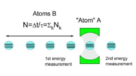
FIG.3 A schematic diagram of the repeated interaction quantum model.The system or“atom” A is represented by a mode in a cavity.A series of heat bath B atoms in the thermal state pass through the cavity and interact with atom A within brief intervals τ.The TEM is applied to each atom B before it enters and after it leaves the cavity.Note that we only record the change in energy and ignore the exact energy values.If this conceptual experiment is conducted over afinite time∆t,the number of B atoms is N= ∆t/τ.These B atoms are composed of Nkatoms at the energy eigenvector|χk〉.

We use a repeated interaction model[5,177−179]to explain QJTs:a quantum system A continuously interacts with a series of atoms B,and these B atoms play the role of the “heat bath”.Fig.(3)is a schematic diagram of the model.Compared with previous models,the model that we are considering is general,and we do not assume that these B atoms are two-level systems(q-bits)[177,178].Before these B atoms interact with the quantum system A,we assume that they are in thermal equilibrium.These atoms then pass through a region wherein they interact with the system or the“atom”A successively forfinite intervals.The global Hamiltonian of the composite A and B atoms is still E-q.(1).We further assume that there are no correlations or interactions among these B atoms.When a B atom enters and leaves the interaction region,its energy is measured,and we record the change in energy.This is simply the TEM scheme applied to the bath atoms.This model is not abstract because many experimental systems can approximately realize it[178].

A.Static Hamiltonian

1.Simple interaction

Wefirst consider the case of the static Hamiltonian with a simple interaction,V=A⊗B,or Eq.(2)witha=1.We suppose that before the interaction with atom B occurs,systemAis initially in a pure state.These two restrictions are based on the following consideration:under this situation,a QJT can be described by the wave vector of the system;otherwise,the density matrix formulation has to be used.Although this is a specific case of the latter,the wave-vector description of QJTs seems to be more accessible to nonexpert readers.In addition,it is easier to realize in numerical simulations as well.We have seen that a major portion of the literature studying SQT using QJTs has favored this formulation[2,5,10,14,16,17,19,20,27].

In analogy to the derivations of MQMEs,our discussion is presented in the interaction picture with respect to the free Hamiltonian,HA+HB.As we have mentioned,before a bath atom B enters the cavity,we measure its energy.Because these bath atoms are in a thermal equilibrium state,the measured atom shall remain at one of the eigenvectors of the HamiltonianHB.Suppose that the wave vector is|χk〉with eigenvalueχk.After a time intervalτ,due to the interaction between the A and B atoms,the global wave vector of the composite A and B system evolves into

where|(t)〉Ais the wave vector of atom A at timetbefore entry of atom B.Because we are using a pertur-

bation approach,we redefineVasαVwith the small parameterα.In the second equation,we collect all terms up to second order inα;all higher order terms are neglected.According to Eq.(34),the interaction picture operatorVis

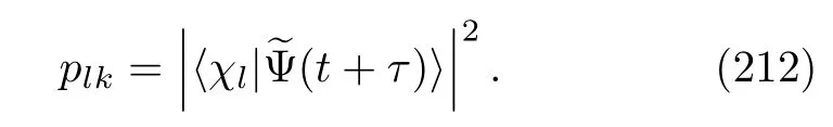
When atom B passes by after a time intervalτ,we measure its energy again.According to the projective measurement assumption in quantum mechanics[180],there are two types of outputs.One output is whereby the measured energy of atom B is stillχk.In this case,the wave vector of atom A after the measurement is

where the coefficientgkis

Noting the presence of the exponential termei(ω−ω′)tin Eq.(207),which is analogous to that in Eq.(123),we may simplify Eq.(207)by applying the rotation wave approximation:

wheregk(τ,ω)is the same as Eq.(208),butωandω′are set equal here.The other possible output is whereby the measured energy value isχl,and especially,l̸=k.In this situation,the wave vector of atom A after this measurement is

where the coefficientflkis

Here,we keep the term of lowest order inα,O(α1).This approximation convention is used throughout this paper,e.g.,Eq.(205).In Eqs.(207)and(210),the coefficientplk(l=korl̸=k)is used to ensure the normalization of the wave vector|(t+τ)〉A,which is

Its concrete expression is temporarily unimportant.

Let us consider a new time scale∆t.We require that it is far larger thanτbut still far smaller than the relaxation time of system A.During this interval,there are many B atoms passing by.Obviously,the number of B atoms isN= ∆t/τ(≫1).We have assumed that the bath atoms are in a thermal equilibrium state.Hence,these atoms are composed of various atoms with energy eigenvalueχk,and in particular,their numbers are

WhenNB atoms pass by,we want to count the energy changes in these atoms.One possibility is that none of the energies change even though they have interacted with system A.In this situation,according to Eq.(209),wefind that the wave vector of system A after the longer time interval∆tis

Notice that we did not yet normalize the vector.Breuer and Petruccione[181]proved that the summation term with respect to the energy quantum numberkis simply

where the functionsrandShave been defined in E-q.(40).To arrive at this result,we have considered that the decay time of the correlation function of the B atoms is far shorter than the interaction time so thatτing(τ,ω)can be replaced by+∞.This is simply the Markovian approximation.Substituting the above result into Eq.(214)and imposing the normalization requirement,we obtain

whereHLShas been given in Eq.(45),and the average〈···〉is with respect to the initial wave vector,|(t)〉A.We have eliminated the parameterαhere.

On the other hand,we mayfind that some B atoms have indeed changed their energies after the time interval∆t.According to Eq.(212),compared with the case of no atoms changing their energies,however,such a probability is very small.Hence,we suppose that,within the time interval∆t,only one B atom changed its energy.Obviously,the choice of∆tbecomes very important to the validity of this assumption.Consider that the energy change is fromχktoχl.The explicit expression of Eq.(211)is

We see that the ratio term on the RHS is a rapidly oscillating and decaying function ofτ;it is significantly non-zero only if

This condition,which we call the energy conservation condition throughout this paper,implies that the major contributions in the sum,Eq.(210),are theA(ω)terms,which exactly satisfy Eq.(218).Conversely,this also indicates that if we really observed an energy change in one B atom within the time interval∆t,its value must be equal to one of the Bohr frequencies.These discussions lead us to the conclusion that the wave vector of system A after an observation of an energy changeωis

The normalization condition has been considered here.We call such a change in the wave vector a jump of typeω.The reader is reminded that as long as oneωis given,although different quantum numbers,landk,(or different wave vectors|χl〉)correspond to different coefficients,flk(τ,ω),they cannot alter the above result due to the normalization.However,if the interaction HamiltonianVis complex,namely,a≥2 in Eq.(2),we cannot obtain the simple Eq.(219).We will discuss this in the next subsection.Because we are only concerned with the energy changeωof the bath atoms and ignore the information of the exact quantum numbersk,our follow-up question concerns the probability of the jump of typeω.After a simple probability argument,we find that it is

Here,the quantum numberlis restricted by the energy conservation condition,Eq.(218).The sum over the quantum numberkis because the jump might occur with every B atom interacting with system A within the time interval∆t.Of course,this is only possible if the energy eigenvalues of the bath atoms are sufficiently dense to satisfy the energy conservation condition.Breuer and Petruccione proved that the above sum term is equal toτr(ω)[181].Hence,Eq.(220)is simplified as

Here,we eliminatedαas well.Although we obtain the probability in the interaction picture,it is the same in the Schr¨odinger picture.

Based on the above discussion,we have a physical picture of the evolution of system A and the energy changes in these B atoms.The B atoms successively pass through the interaction region,and we continue recording their energy changes.At each time intervalt～t+∆t,we have the probability

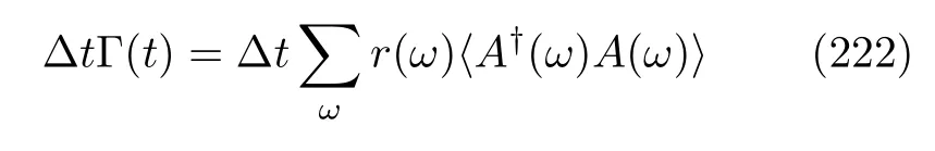
offinding that an energy change has occurred.Obviously,Γ(t)has an interpretation of being a total instantaneous jump rate.If a jump of typeωis indeed recorded,the wave vector of system A is updated to the new wave vector,Eq.(219).Because the probability is very small,we more often see that there is no change in the energy.In this situation,system A deterministically evolves according to Eq.(216).These two types of evolutions alternatingly proceed until the process is terminated at the end timetf.We call the full evolution ofa QJT in the system’s Hilbert space and denote it as.

Eqs.(216)and(219)can be written in a concise form:

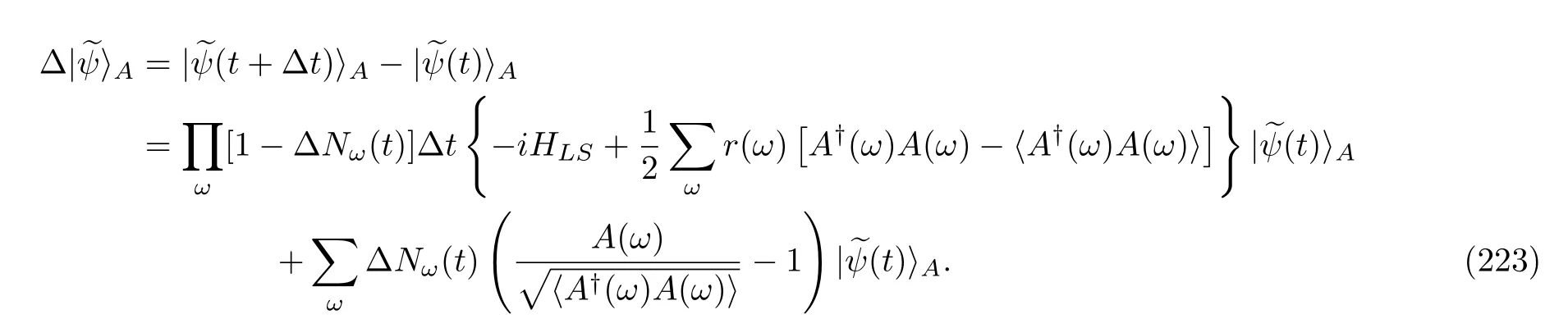
The stochastic variable∆Nω(t)is equal to 1 or 0 with corresponding probabilitiesPω(t)or 1−Pω(t).Obviously,its average is

The reader is reminded that the above average is performed over a given|(t)〉A.Hence,it is a conditional average.On the other hand,we may re-express E-q.(223)using the density matrix formula

It is straightforward to prove that

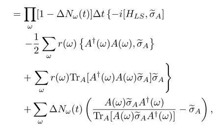
We also call the time evolution ofAa QJT in the system’s density matrix space and denote it as{A}.The reader is reminded that Eq.(226)can be obtained by applying the density matrix formula at the beginning rather than being indirectly derived from the wave vector.Although Eqs.(226)and Eq.(223)are equiv-alent to each other,we will see that only the former form can be extended to situations with the general system’s initial conditions and/or with a complex interaction Hamiltonian.

Let us discuss several consequences of the QJT concept.First,a QJT is combined with alternating deterministic evolution and stochastic jumps.Hence,QJTs are typical piecewise deterministic processes(PDPs)[78]concerning the wave vector or density matrix of system A.One can study the dynamic equations of their distribution functions based on the standard theory of PDPs.We refer the interested reader to the textbook by Breuer and Petruccione[78].Second,a QJT is a random process.For each realized process,the density matrixA(t)at a given timetis random.One may prove that its mean over all processes,

satisfies a time evolution equation:

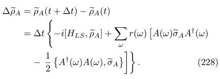
As∆tgoes to zero,the above equation is simply the MQME for the static Hamiltonian in the interaction picture,Eq.(44).Notice that the mean(227)is not the same as the conditional average(224).To obtain Eq.(228),we have used a key identity[98],

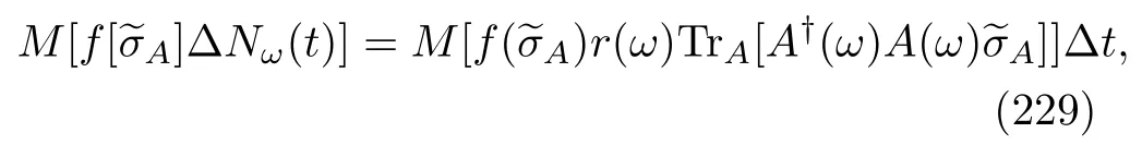
wherefis an arbitrary function ofA.The reason for Eq.(229)is simple:the probability offinding a specificAand∆Nω(t)equals a multiplication of the probability offinding the density matrix and the conditional probability offinding∆Nω(t)givenA,where the latter is simplyPω(t),Eq.(221).Finally,we can simulate Eqs.(223)or(226)using a Monte-Carlo method.According to Eqs.(221)and(222),the probability of observing a deterministic evolution from timet′untiltand then being interrupted by a jump of typeωduring the time intervalt～t+∆tis

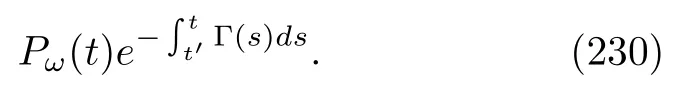
Hence,we can construct the probability offinding a QJT that starts at time 0,jumpsNtimes with typesωiat time intervalsti～ti+ ∆ti(i=1,···,N),and ends at timet:

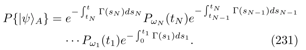
This formula is very analogous to the probability of observing a classical jump trajectory in discrete state space[89].We can also write the above probability alternatively using the density matrix of the QJT:

where the superoperatorsJ(ω)are defined as

andG0(ti,ti−1)(i=1,···,Nandt0=0)is the superpropagator of the time evolution equation,

namely,

We have transformed back to the Schr¨odinger picture.Both superoperators act on the symbols on their RHSes.Note thatπA(t)is not yet normalized.An explanation for the equivalence of Eqs.(231)and (232)is given in Appendix E.We will see that these two equations,especially the second equation,play central roles in deriving various FTs at the QJT level.

2.Complex interaction

Here,we want to extend the previous results to the case of the general interaction Hamiltonian,Eq.(2)(a≥2).Wefirst concretely explain why the wavevector description of QJTs fails even if the initial state of system A is a pure state.If the initial state is a general mixed state,the failure is apparent.Assume that at timetthe wave vector of system A is|(t)〉A.We can perform an analogous analysis to that performed previously and find that,after the time interval∆t,if an energy changeωoccurred at one B atom,the system state is updated to

where the energy conservation condition,Eq.(218),has been considered due to the coefficient

The presence of the sum over the indexais due to the fact that,given the same Bohr frequencyω,there are several different corresponding operatorsAa;also see Sec.(II.B.1).Obviously,for different quantum numbersl,the wave vector Eq.(236)is distinct even if the types of jumps are exactly the same.Because we do not record the concrete quantum number that is in charge of the jump,the density matrix formula is naturally needed.To this end,consider the density matrices of a B atom and of system A to be|χk〉〈χk|andA(t),respectively.The global density matrix of the combined A and B systems after a brief interaction timeτis

Then,we measure the energy of the output B atom.If the atom remains at the same eigenvector with eigenvalueχk,the density matrix of the system A is then

where

To be similar with the previous argument,according to the rotating wave approximation,we may simplify Eq.(239)by keeping all terms withω=ω′.In particular,within a longer time interval∆t,in which there areN(≫1)B atoms interacting with system A,if we do not observe a change in energy of these B atoms,we find that at timet+∆tthe system’s density matrix evolves to

Substituting this into Eq.(241)and normalizing,we obtain

The other possible output is that there is an energy change at one of these B atoms.Let us again suppose that the change in the energy of the B atom isωand that this has occurred from an eigenvalueχktoχl.In this situation,the density matrix of atom A jumps to

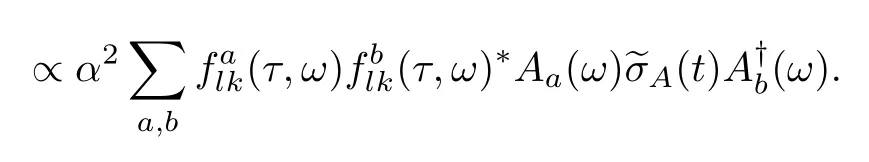
We have considered the energy conservation condition Eq.(218).Obviously,the density matrix after the jump depends on the concrete quantum numberk.Because we only record the change in energyωinstead of the exact quantum numberk,the genuine density matrix at timet+∆tshall be a sum of the weighted density matrix with a specifickvalue,namely,

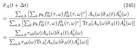
This density matrix has been normalized.To derive the second equation,the following identity was used[181]:

According to Eq.(245),we see that the possibility offinding such a change in energyωis

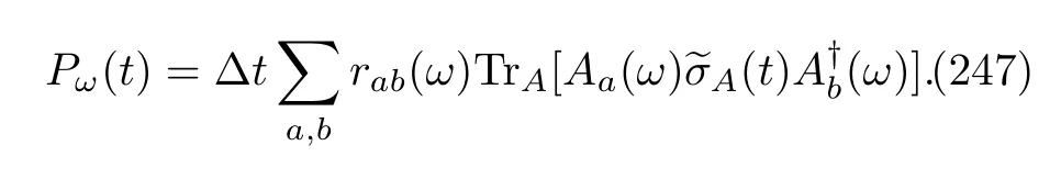
Hence,the probability of observing an energy change during a time intervalt～t+∆tis

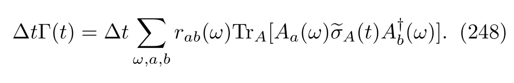
We can combine Eqs.(243)and(245)into a compact form:

where∆Nω(t)is also a stochastic variable,equal to 0 or 1,and

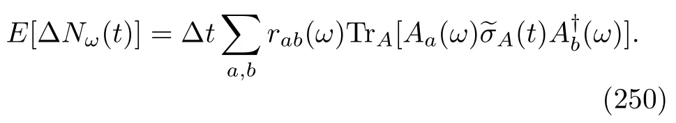
We call the density matrix evolution described by E-q.(249)a QJT in the system’s density matrix space.Analogous to the case of the simple interaction Hamiltonian,if we perform an average of Eq.(249)over all QJTs,we canfind that the mean,

satisfies the time evolution equation

where we have used an extension of Eq.(229):

Eq.(252)is simply the MQME for the static Hamiltonian in the interaction picture or Eq.(124)withη=0.

Eq.(249)can also be simulated by the Monte-Carlo method,which is almost the same as that in the preceding subsection.In particular,the probability of observing a trajectory is also described by Eq.(231)or(232)except thatPω(t)is equal to Eq.(247)instead of(221),where the superoperator

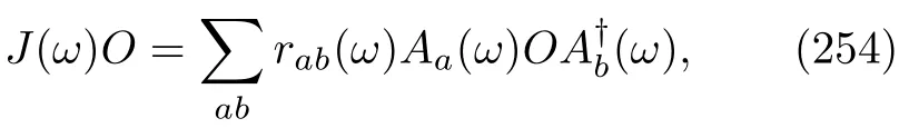
andG0(ti,ti−1)is the superpropagator of the following equation:

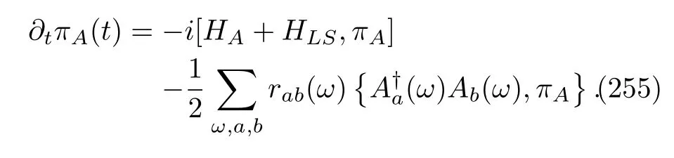
Note that we have transformed back to the Schr¨odinger picture here.Obviously,if both the subscriptsaandbare equal to 1,all the results in this subsection are reduced to those in the case of the simple interaction Hamiltonian.Finally,we want to emphasize that our treatment of the repeated interaction quantum model and the explanation of the QJT concept is not very rigorous.For instance,we did not clarify how choosing∆tmakes it far larger than the brief interaction time intervalτwhile ensuring an energy change has only occurred at one B atom.We refer the interested reader to a rigorous theory of the quantum model given by Attal and Yan[179].

B.Other time-dependent Hamiltonians

In this section,we want to generalize the previous results in the static Hamiltonian case to the cases of time-dependent Hamiltonians.From the above discussion,we noted that there is no fundamental differences in the spirit of obtaining the QJT concept in the cases of simple or complex interaction Hamiltonians,although the latter are indeed more complicated notationally.Hence,for the sake of simplicity,the results for the cases of time-dependent Hamiltonians that we are presenting are only for the case of simple interactions.

1.Weakly driven Hamiltonian

The Hamiltonian of the quantum system A is E-q.(48).Becauseγis a small parameter,we may take a Taylor series for Eq.(206)atγ=0 up to zeroth order:

The reader is reminded again that hereA(ω)is the decomposition with respect to the eigenvectors and eigenvalues of the bare HamiltonianH0.Because we have assumed that the magnitude ofγis the same as that ofαand because we only consider the lowest order approximation,most of the formulas in this case are retained except that,in Eqs.(234),HAis changed into the weakly driven Hamiltonian,Eq.(48).

2.Periodically driven Hamiltonian cases

For the periodic Hamiltonian,Eq.(50),based on Eq.(56),the key interaction picture operator forVis

When we compare Eqs.(257)and(206),wefind that they are almost identical in form.Hence,without further derivations,in this case,we conclude that the QJT concept and its physical interpretation can be well established,as we did in the case of the static Hamiltonian,and previous formulas are also retained without significant revisions.The reader is reminded that the parameter 0 inA(ω,0)is essential if one wants to obtain formulas in the Sch¨odinger picture;see Eq.(61).

3.Adiabatically driven Hamiltonian case

This case is slightly complicated.According to E-q.(64),the interaction picture operator ofVis

where the decompositionAnm(t,0)depends on timet,which is significantly distinct from the previous three cases. Substituting it into Eq.(205),if no energy change has occurred at a B atom staying at the state|χk〉,the wave vector of the quantum system A after the second energy measurement is then

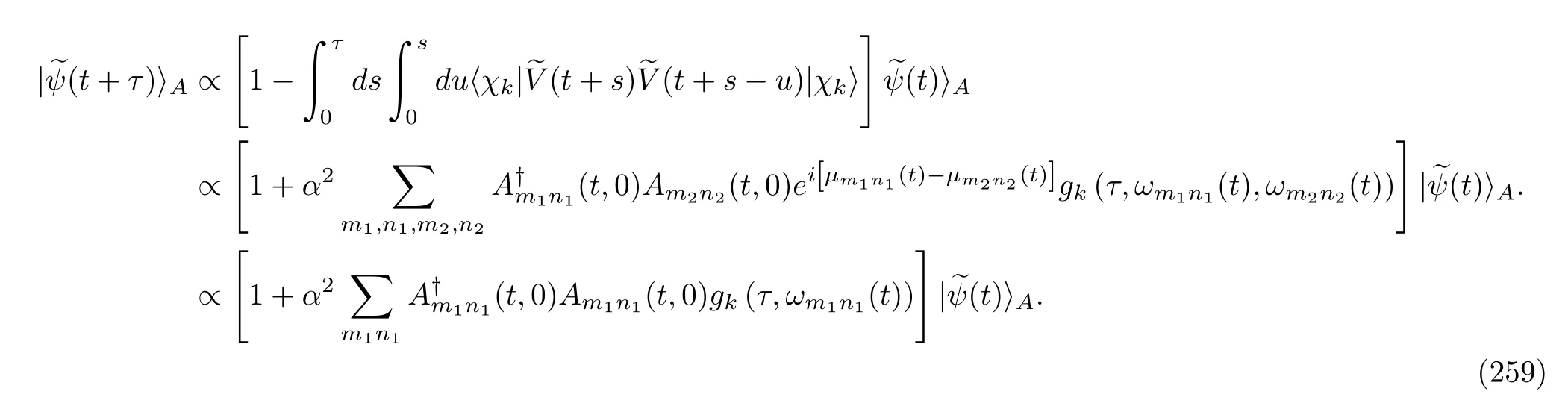
To obtain the second equation,we have regardedsands−uas small parameters and used the approximation in Eq.(71).The last step is due to the application of the rotating wave approximation.If we further consider the influence ofNsuccessive interactions between the system A and B atoms within the time interval∆t,because the external protocol varies slowly(adiabatic approximation),we may reasonably suppose that the time parametertin the last equation of Eq.(259)isfixed.Hence,in this case,we still obtain an evolution analogous to Eq.(216)except thatA(ω)therein is replaced byAm1,n1(t,0)and that the sum is aboutm1andn1rather thanω.On the other hand,if a B atom changes its energy from eigenvaluesχktoχlafter a brief interaction with system A,the wave function of the system jumps to

We have noted that the coefficientflkis significantly non-zero only when the condition of energy conservation is satisfied.In the current case,the condition is

Because we have assumed thatωmn(t)corresponds to a unique set of quantum numbers(m,n)(see Sec.II.B.4),the above energy conservation condition indicates that there is only one term remaining in the sum of E-q.(260).Hence,for the case of an adiabatically driven Hamiltonian,we still obtain a jump in the wave vector of the system as Eq.(219)except thatA(ω)therein is replaced byAmn(t,0).

C.QJT for the general MQME

We have explained the QJT concept for several open quantum systems.Therefore,could we have a unified approach to obtain these results in a more ef-ficient manner?We hope that this approach could be directly performed on general MQMEs,Eq.(77).This may then provide convenience when we discuss the QST of QJTs from a general perspective.Such a type of approach indeed exists and was mainly developed by Srinivas and Davies[94],Carmichael[96],Wiseman and Milburn[91],and Kist et al.[177].However,their discussions were limited to time-homogenous MQMEs.Here,we will show that their ideas can be easily extended to the time-dependent situation.

Wefirst rewrite the general equation(77)in the following form:

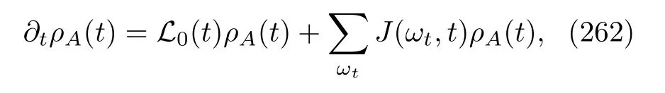
where these two superoperators are defined as

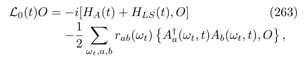
and

respectively.Now,treating theseJ-terms as“perturbations”,we can obtain its Dyson series solution,

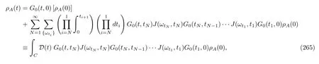
where{ωti}={ωtN,···,ωt1},the sums are over all possibleωtiat timestiordered byt=tN+1≥tN≥t1≥0,and the propagator is

The reader is reminded that these superoperators act on all terms on their right-hand side.For simplicity,we used the abbreviationD(t)and the subscriptCto denote that these integrals and sums are with respect to all possible arrangements.

Atfirst sight,the physical relevance of this integral formal solution is ambiguous.After all,the decomposition of Eq.(262)is non-unique.However,we see that the integrand in Eq.(265)is very similar to the whole term in the trace of Eq.(232).Indeed,for the case of static Hamiltonians with a simple interaction Hamiltonian,the superoperatorsL0andJin Eqs.(263)and(264)are reduced to those in Eqs.(233)and(234).In particular,according to Eq.(347)in Appendix E,wefind that

whereσA(t)is the density matrix of the system along the trajectory{σA}at timet,and the probability of observing a QJT,P{σA},has been given by Eq.(232).Hence,the RHS of Eq.(265)is a weighted sum over all possible QJTs of the open quantum system A,and the Dyson series solution is simply

or the Schr¨odinger picture of Eq.(251).Although our current discussion is on the static Hamiltonian case,the results are relevant to other MQMEs as well.The interested reader may check them individually.Finally,we shall note that the trace of the integrand in Eq.(265),

has the interpretation of a probabilitydensityof observing a particular QJT in the density matrix space of the system:it has an initial density matrixρA(0),which undergoesNjumps at increasing timesti(i=1,···,N),with an order of jump types{ωti}.

VII.TRAJECTORY HEAT AND WORK

The previous discussion has clearly shown that the presence of QJT is due to the fact that some external detector is continuously monitoring the changes in energy of the bath atoms:within a time intervalt～t+∆t,if the system A evolves deterministically,there are no energy changes characterizing these passing B atoms;on the contrary,if the state of system A jumps,an energy change,ωt,essentially occurs at one of these B atoms;see the energy conservation condition,Eq.(218).Hence,given a QJT{σA}within a finite time interval,(0,tf),if we record all these energy changes(not the exact energy values of these B atoms)and sum up these numbers,we will obtain the total energy exchanged between the single open quantum system A and the bath B atoms.From the perspective of thermodynamics,we naturally interpret this exchanged energy as the heat released along the QJT.Hence,given that there areNjumps of typeωti(i=1,···,N),the trajectory heat is formally defined as[2,10,14,17,20,27,92,93,100]

Note that we do not impose any restrictions on the initial density matrix of the system,σA(0).

We may also define the trajectory work.In contrast to the trajectory heat definition,we have to apply the TEM scheme[65,71]to the single system A in addition to continuously monitoring the energy changes in these B atoms.Because the energy measurement is performed on system A at the beginning,its initial density matrix is no longer arbitrary.This is the same as what we have considered in Sec.IV.A.Assuming that the system’s HamiltonianHA(t)has instantaneous eigenvectors|εn(t)〉with discrete eigenvaluesεn(t),for a QJT{σA}withNjump types{ωti},starting from the density matrix|εm(0)〉〈εm(0)|and ending at the density matrix|εn(tf)〉〈εn(tf)|,because of the last energy measurement at the end timetf,the trajectory work is defined as

Obviously,this is the inclusive work at the trajectory level and is thefirst law of thermodynamics under the concept of QJTs.In addition,if the open quantum system has the Hamiltonian in Eq.(107),we may alternatively define the trajectory exclusive work if the TEM is applied to the bare Hamiltonian,H0.In this case,the exclusive work is

whereεnandεmare the energy eigenvalues ofH0.

VIII.TRAJECTORY CHARACTERISTIC OPERATORS

Obviously,the trajectory heat and work,E-qs.(270)-(272),are random due to the random characteristics of QJTs.Hence,it shall be interesting to explore their statistical features.In particular,because QJTs have very strong connections with the MQMEs,one may naturally speculate that their statistics should consist of those of the stochastic heat and work defined by applying the TME scheme to the combined system and heat bath;see Eqs.(99),(102)and(108).However,there are no ad hoc reasons to support this conjecture.After all,very different measurement schemes are involved in these two types of stochastic thermodynamic quantities.Because the QJT has a classical probability measure,we can also define the CFs for the random trajectory heat and work in analogy to what we did in Sec.IV.For the heat case,its CF is apparently

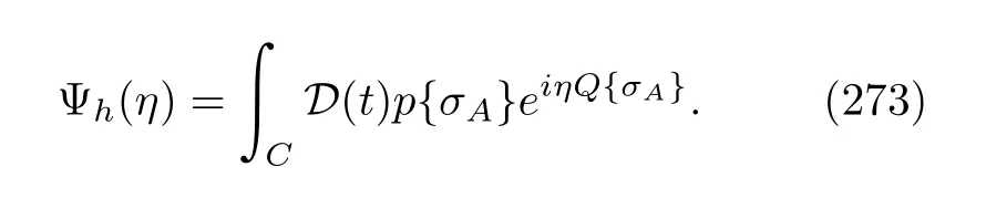
Substituting Eqs.(269)and(270),the RHS of the above equation becomes

We immediatelyfind that the entire term in the square brackets is almost the same as the Dyson series solution,Eq.(265),for the general MQME;the only difference is that each superoperatorJ(ωt,t)in the latter is multiplied by an exponential“phase” factor,eiηωthere.Hence,without further derivations,this analogy leads us to conclude that,if we define the whole integral in Eq.(274)as the trajectory HCO,it must satisfy a time evolution that is exactly the same as that ofA(t,η);see Eq.(125).Therefore,we do not need to introduce new notation for the trajectory HCO.In a word,we have confirmed the conjecture in the heat case.The reader is reminded that during the construction of the QJT concept,we implicitly applied the weak coupling limit.For instance,Eqs.(209)and(215)achieve rigorous mathematical meaning only in this limit.Hence,the statistics of the stochastic heat and work are defined by either the TEM scheme on the composite system or the QJTs having the same mathematical foundation.It would be interesting to say some words about the history of Eq.(125)[31,97].Although this result was usually attributed to Espositor[4],the earliest version shall be credited to Mollow[110],who investigated the probability distribution of the number of photons of a two-level atom that is driven by a weak classicalfield and simultaneously interacts with a bath of modes of a radiation field.Zoller et al.[111]extended Mollow’s result to three-level systems.At that time,the concept of QJTs was still in its infancy,and the emission and absorption of photons were not interpreted as heat.

The next thermodynamic quantity is the trajectory work,Eq.(271).Its CF is

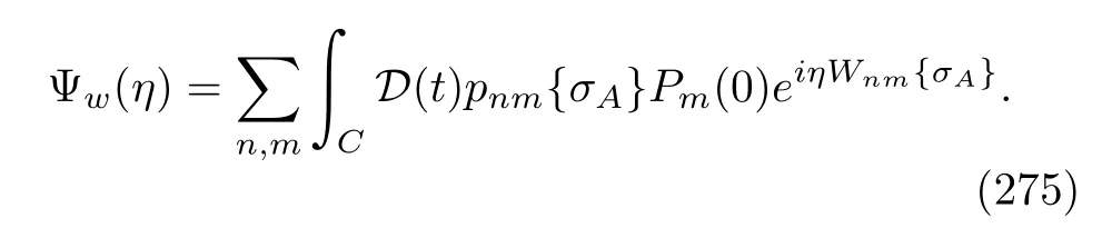
wherePm(0)is the probability of observing the quantum system A at the eigenvector|εm(0)〉,and the probability density of observing a QJT that has an initial density matrix|εm(0)〉〈εm(0)|,that undergoesNjump-s at increasing timesti(i=1,···,N)with an order of jump types{ωti}and that is measured to be at the energy eigenvector|εn(tf)〉〈εn(tf)|at timetfis equal to

To obtain the second equation,we have used Eq.(267).SubstitutingEqs.(271)and (276)into Eq.(275),we immediatelyfind that its RHS is equal to

where the initial density matrix is

We have assumed that this is indeed the initial density matrix of the quantum system A and that it is not affected by the first energy projection measurement.In comparison with Eq.(274),in addition to the fact that the initial density matrix is replaced bye−iηHA(0)ρA(0),the other difference is the presence of an operatoreiηHA(tf).Therefore,we find that the whole term in the trace of Eq.(277)is simply the whole term in the trace of Eq.(129).Specifically,it is exactly the same as the WCO,KA(η,tf).Therefore,analogous to the heat case,we do not need to define the trajectory WCO at all.Note that all these discussions are also relevant to the case of the trajectory exclusive work,Eq.(272).We do not write them here.

Based on the above discussion,we arrive at the following important conclusion:for all MQMEs that we discussed so far,the stochastic heat and work,which are defined either by the TEM scheme applied to the combined system and heat bath or at the QJTs,their statistics are indeed exactly equivalent.This conclusion has two important consequences.On the one hand,this equivalence reminds us that we may measure these thermodynamic quantities experimentally by these two seemly very distinct measurement approaches.So far,we have not been very clear on how to realize the TEM measurement for the heat and work experimentally,even though their definitions are very simple and straightforward.On the contrary,QJT experiments have become a reality[163−172].On the other hand,from a computational perspective,we can calculate the distributions of these thermodynamic quantities either by numerically solving the time evolution equation,e.g.,Eqs.(125)or(130),and then performing a Fourier inverse transformation,or by performing a Monte-Carlo simulation.In many cases,the former is analogous to solving the evolution equation of the density matrix Eq.(77)of an open quantum system.Suppose that the Hilbert space of the system has dimensions ofD.The number of variables of the matrices,A(t,η)orKA(t,η),isD2.In contrast,the number of variables involved in the Monte-Carlo method when solving the wave function evolution,Eq.(223),isD.Hence,if the dimensionDis very large,the required computational resources of the Monte-Carlo method increase as～D,which is substantially smaller than the requirement of solving the evolution equations,i.e.,～D2[78].

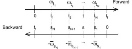
FIG.4 A QJT of the forward MQME(the upper line)a nd its backward trajectory(the down line). The arrows indicate the time directions of the evolutions.The jump types of the forward QJT are ordered by increasing times as ωt1,···,ωtN.Then,the corresponding jump types of the backward QJT are ordered by increasing time as−s1,···,−sN,where si= ωtjwith si+tj=tfand i+j=N+1.

IX.TRAJECTORY FLUCTUATION THEOREMS

Because the time evolution equations of the trajectory HCO and WCO are still Eqs.(125)and(130),respectively,their CFs of course satisfy the same symmetries as those in Sec.V.B.Furthermore,the establishment of the QJT concept implies that there exist new FTs at the trajectory level.In classical ST,trajectory FTs are well known,e.g.,the total entropy production FT[59].Horowitz and Vaikuntanathan[180]even generalized these FTs to the case in the presence of feedback.In the quantum regime,very analogous efforts have been made by Crooks[7],Horowitz and his colleagues[5,10,23,112].In this section,we want to present the trajectory versions of several previous FTs.Thefirst version concerns the ration of the probability densities of observing a forward QJT to a backward QJT:

where the forward trajectory{σA}comes from the forward QME(77)with an assigned initial density matrix,the completely random matrixC. The backward trajectory comes from the backward MQME,i.e.,Eq.(186)with vanishingη. Assume that the QJT{σA}hasNjumps with increasing time order-Its backward trajectoryis then also started from the completely random matrixCbut consists ofNjumps with increasing time order(see Eq.(194))and particularly

withi+j=N+1(i=1,···,N).According to our previous convention,the parameterswas used to denote the time of the backward process.

To prove Eq.(279),let us define the duals for the superoperatorJand the propagatorG0in Eqs.(264)and(266):

where

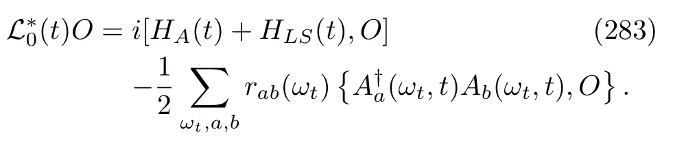
The definition of the dual was given in Eq.(188).On the other hand,we note that,if we apply adjoint transforms to these superoperators,we have

Under these notations and formulas,we can rewrite the probability density of the forward QJT,Eq.(269),as

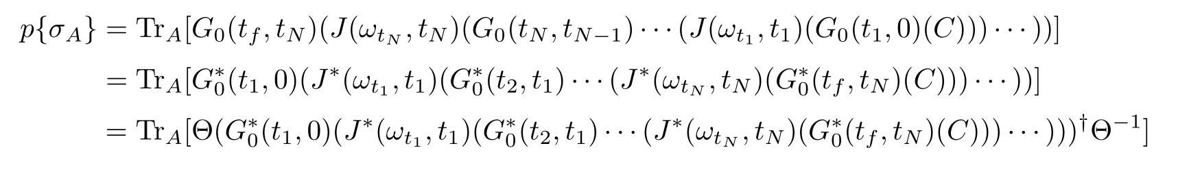
We have added circle brackets to clarify the acting regime of each superoperators.

To connect this result with the backward QJT,we still need two additional formulas.Thefirst formula concerns the superoperator ofJ:

whereis the J-superoperator but of the backward MQME,that is,

The proof is straightforward if we apply the KMS condition,Eq.(43),and Eqs.(193)-(195).The other formula is

wheretj−1≤t≤tj,si≤s≤si+1,t+s=tf,andG0(s,si)(si≤s)is the propagator of the deterministic evolution of the backward process.The proof of Eq.(289)is very similar to that of Eq.(191).Let the LHS of Eq.(289)beWe then take a derivative with respect to timesand obtain

The last equation was obtained by inserting the explicit formula forand applying Eqs.(193)-(195).This is clearly the continuous evolution equation of the backward MQME.Considering the initial condition,we have proved Eq.(289).

Now,we are in a position to prove the trajectory FT for the heat.By repeatedly applying Eqs.(287)and(289)to Eq.(286),we immediatelyfind that the original one is equal to

The trace term on the RHS is simply the probability densityof observing the backward QJTof the backward process.Therefore,we have proved Eq.(279).

We can consider analogous discussions for the cases of trajectory inclusive and exclusive work.Wefirst notice that the trajectory probability density,Eq.(276),can be rewritten as

On the RHS,is the probability density of observing the backward trajectory that initially starts from the energy eigenvector|εn(tf)〉,withNjumps with time orderand is measured to be at the energy eigenvector|εm(0)〉at the end timetf.Note that we have assumed thatHA(t)is TRI;see Eq.(181).Based on this equality,we further have

wherePm(t)=e−βεm(t)/Z(t)andt=0,tf.Obviously,the numerator on the LHS is the joint probability of measuring system A at the eigenvector|εm(0)〉at time 0 and the QJT being{σA}.The denominator has the same meaning but is initially measured at the eigenvector|εn(tf)〉and concerns the backward process.BecausePm(0)andPn(tf)have canonical distributions,the initial states of these two processes are in thermal equilibrium with the heat bath at the inverse temperatureβ,and in particular,their Hamiltonians areHA(0)andHA(tf),respectively.An analogous formula can also be derived for the trajectory exclusive work:

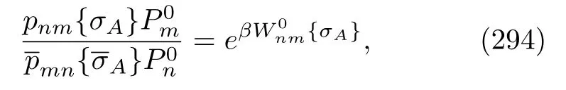
X.TOTAL ENTROPY PRODUCTION

In addition to the stochastic heat and work,the total entropy production(TEP)is also an important thermodynamic quantity in irreversible thermodynamics[81].In the classical situation,it has been well established that the TEP can be defined at the classical trajectory level,and in particular,it also satisfies intriguing FTs[55,59].It shall be interesting to investigate their correspondence to MQMEs.Analogous to the cases of heat and work,we can realize this aim through two methods:one method is based on an analogous TEM scheme but one not acting on the system’s energy,and the other method is to define a TEP along a QJT.Because the whole consideration is very similar to the cases of heat and work,our discussion about the TEP is brief.

The density matrix of the open quantum system is Hermitian.It possess a diagonal form in its instantaneous orthogonal basis|ρµ(t)〉.Specifically,we suppose that the spectral decomposition of the density matrix is

The eigenvalueρµ(t)has an interpretation that it is the probability offinding the system at the eigenvector|ρµ(t)〉.To define a stochastic TEP,we measure the instantaneous eigenvector|ρµ(t)〉and energy eigenvector|χl〉of the open quantum system A and heat bath B,respectively,at the beginning and end of the non-equilibrium process.Then,the stochastic quantity is

Here,we have assumed that these algorithm functions are well-defined,orρµ(t)＞0.Note that Eq.(296)is usually distinct from the classical Shannon entropy[59]:here,−kBlnρµ(t)is related to the von Neumann entropy,and these two types of entropy are not essentially the same[78].The above definition is very analogous to the definition of the inclusive work,Eq.(102).Hence,this similarity leads us to obtain the CF of the TEP of the open quantum system A:

Obviously,choosingη=i/kBand considering E-q.(172),this CF is simply equal to 1.Therefore,the integral FT of the TEP is established as follows:

In contrast to the previous FTs for heat production and work,the current FT is true for very general initial conditions.Hence,we did not add any subscripts in this equality.According to Jensen’s inequality,Eq.(298)implies that〈S〉≥0,or the second law of thermodynamics for the general MQME,Eq.(77).Spohn[82]and Spohn and Lebowitz[81]presented a general formula of the TEP for an arbitrary time-homogeneous quantum dynamical semigroup having a stationary state.In this specific situation,our results are consistent with their formula.

On the other hand,for a QJT that starts from an initial density matrix|ρµ(0)〉〈ρµ(0)|,jumpsNtimes with typesωti(i=1,···,N),and ends at|ρν(tf)〉due to the second measurement of the system at timetf,we define its trajectory TEP as

Eq.(270)presents the explicit expression forQ{σA}.We can write the probability density of observing such a QJT as

Furthermore,we have the following trajectory FT for the TEP:

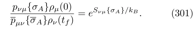
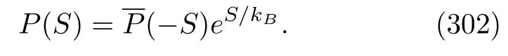
The reader is reminded that the initial density matrix for the backward MQME is ΘρA(tf)Θ−1.

XI.EXAMPLE:PERIODICALLY DRIVEN TWO-LEVEL SYSTEM

Several simple models have been used to illustrate the computations of distributions of the stochastic heat and work and their FTs[10,16,17,19,20,24,25,27,118].A major portion of them are two-level systems(TLS),including cases of being driven by a weak externalfield,adiabatical externalfield,and periodical externalfield.In this section,we want to use the last model to show the computation of the inclusive work distribution.On the one hand,the thermodynamics of this model at the ensemble level has recently attracted substantial interest[85,105,135,136].On the other hand,to the best of our knowledge,whether there is the JE in this system has not been definitively answered in the literature.Although we have formally proved that the equality is true,it shall be more desirable to obtain numerical verifications.Finally,using this non-trivial model,we also want to show the reader the consistency of the two methods in computing work distributions:one method is a direct simulation of QJTs,and the other method is to solve the time evolution equations for the HCO and then to perform a Fourier inverse transform of the CF.

The TLS Hamiltonian is

whereω0is the frequency of transitions between these two levels,Ω is the Rabi frequency,andωLis the frequency of the periodic externalfield.We can analytical-ly solve for the Floquet basis of this system[104,105,136]:

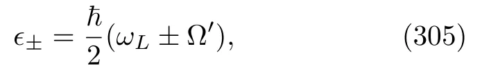
respectively.Assume thatωL−Ω′＞0 and that the coupling between the TLS and heat reservoir is transverse[104,105,136],namely,A=σxin the interaction HamiltonianV.In this case,there are a total of sixA(ωt,t):Three of them are

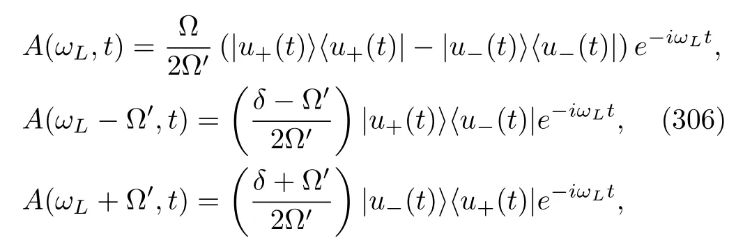
and the other three operators areA(ωt,t),whereωt=−ωL,−(ωL−Ω′),and−(ωL+ Ω′)are the adjoint operators of Eq.(306).Note that theseωtare time independent.Assuming that the bath is composed of an electromagneticfield in thermal equilibrium at a certain temperatureTand that the coupling between the TLS and the reservoir is a dipole interaction,the Fourier transforms of the bath correlation function have the following standard form[78,105]:ifω＜0,

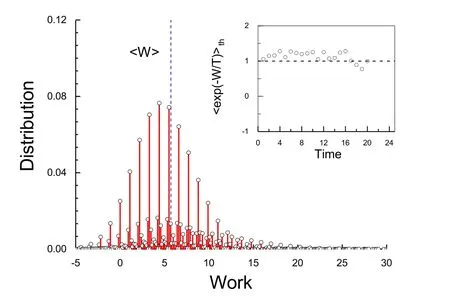
FIG.5 The distribution of the inclusive work(in units of ħω0)in a periodically driven TLS at timeWe calculated it by simulating the QJTs.The initial density matrix is set to be the thermal equilibrium state at temperature T.The utilized parameters are ωL=1.1ω0,Ω =0.8ω0,For convenience,we have let kB=1,ħ =1,and ω0=1.The inset shows the results of the RHS of Eq.(174)calculated at different times through simulation.The dashed line therein is provided as visual guidance.We have used the same model and the same set of parameters to investigate the heat distribution and the heat equality,Eq.(173)[118].

otherwise,ω＞0,and using the KMS condition,r(ω)=eħω/kBTr(−ω),where the coefficientAdepends on the dipole strength.At the initial time,we assume that the TLS is in a thermal state with temperatureT.

Using the Monte-Carlo technique[78],we may easily realize the QJT simulation and construct histograms for the inclusive work after collecting adequate data.The simulation details are presented in Appendix F.Fig.(5)illustrates a distribution at a specific time under a given set of parameters.We see that the distribution is complex,although the model seems to be a simple TLS.To verify the JE,we need to simulate a series of work distributions at different times and then calculate the LHS of Eq.(174);see the inset of the samefigure.Note that the ratio of the partition functions of the RHS of the same equation is 1 and is independent of time.We see that Eq.(174)is satisfactory,although there are apparent deviations at certain times.We attribute these deviations to statistical errors due to thefinite number of QJTs.To show the consistency of the two methods in computing the inclusive work distributions,we calculate Eq.(129)by numerically solving the time evolution equation(125),performing an inverse Fourier transform and comparing the obtained probability distribution to that obtained by direct simulation2We may as well solve Eq.(130)for KA(t,η)and then obtain the CF, Φw(η)=TrA[KA(tf,η)].This is true in principle.However,we have to face an additional difficulty in the numerical realization of the term ∂t[eiηHA(t)]e−iηHA(t).We have met an analogous problem in the quantum piston model;see Fig.(1).However,considering that we had the probability distribution,it is obviously easier to make it a Fourier transform and to compare the result to the CF obtained by solving Eq.(125).We did this when we considered the inclusive work distribution in the quantum piston model;see Sec.III.Fig.(6)shows the CFs obtained by these two routines,where the work distribution is that shown in Fig.(5).The computational details of solving the time evolution equation are also presented in Appendix F.We see that these two CFs are in excellent agreement with each other.Because in the current case the time evolution equation has an exact solution,the small differences between the two results shown in Fig.(6)are from the statistical errors of the QJT simulations.

FIG.6 The CFs calculated by simulating the QJT method(circles)and by solving the time evolution Eq.(125)(curves).The former is obtained by performing the Fourier transform on the work distribution shown in Fig.(5).The computational parameters are the same as those previously used.

XII.DISCUSSION AND CONCLUSION

In this paper,we reviewed the stochastic heat and work in MQMEs and two strategies of studying them.One strategy is to treat the system and its surrounding heat bath as a closed quantum system;the evolution of the composite system is unitary under the control of a time-dependent total Hamiltonian,and the heat and work are defined as the changes in energy by the TEM scheme applied to the composite system.The other strategy is to unravel these MQMEs into QJTs,and the stochastic heat and work are defined along the individual trajectories.Our results clearly show that these two strategies lead to the same statistics for these thermodynamic quantities,although their definitions are based on these seemingly very distinct measurement approaches.It is useful to summarize the advantages of these two strategies.Although thefirst strategy is based on the idea of quantum master equations,because the physical picture of the composite system is always meaningful,this strategy can be extended in a straightforward manner to more complex situations,e.g.,strong interaction between quantum systems and their environments and non-Markovian behaviors.The second strategy would be more attractive if we were given an MQME in advance.We have observed that a QJT has an intuitive physical explanation;its mathematics is simple and easily simulated by computers,and in particular,it is more realistic experimentally.

Let usfinish this paper by pointing out several extensions.Thefirst extension is to study scenarios containing multiple reservoirs or particle transport.So far,we have only been concerned with one heat bath with a thermal temperature,and particle exchange is not allowed.Some studies have already considered this issue[4,25,29,74,105].However,few studies have applied the concept of QJTs.The second possible extension is to account for non-Markovian effects[140,184,185].Non-Markovian properties usually lead to a failure of the MQME(77),on which we heavily rely.However,the extension of the state space of an open system may retrieve this key form[140,184].It would be interesting to determine what type of role the KMS condition plays in QST in this situation. Finally,the role of the many-body interactions of the quantum system in ST is a very intriguing issue.Some studies have shown that QJT could be very useful in studying this issue[186].

ACKNOWLEDGMENTS

This work was supported by the National Science Foundation of China under Grant Nos.11174025 and 11575016.We also appreciate the support of the CAS Interdisciplinary Innovation Team,No.2060299.

APPENDIX A:FEYNMAN-KAC FORMULAS

In 1947,Kac[150]proposed the following question:Given a functional

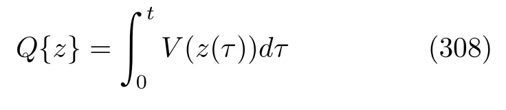
of a classical Brownian process{z},becauseQis a random variable,how can one calculate its distributionp(Q)?Rather than on the distribution itself,Kac focused on its moment-generating function(MGF)3The moment-generating function is the Laplace transform of probability distributions,rather than the Fourier transform used in CF.However,if all the moments of a stochastic quantity exist and are finite,there are no essential differences between two functions;a moment-generating function may simply be regarded as a CF evaluated on the imaginary axis[125].If onefirst calculates the MGF,the distribution can be obtained by taking an inverse Laplace transform.,or

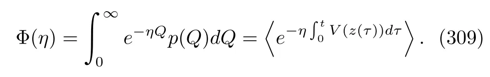
The last equation indicates that the average is taken over all Brownian stochastic trajectories,which possess probability weights.He found that this MGF can be calculated by an integral of a functionG(z,t),namely,

while the functionGsatisfies a partial differential equation given by

whereDis the diffusion constant.The above three equations are collectively known as the celebrated FK formula[188].The formula indicates that if we could solve Eq.(311),after integrating the solution overzand inverting the Laplace transform Eq.(309),we can obtain the distributionp(Q).

FK has numerous applications in diversefields[189];it also has many extensions.One such extension that is relevant to us is that the Brownian diffusion can be replaced by a deterministic dynamics controlled by a HamiltonianH(z,t).In this situation,Eqs.(308)-(311)remain valid except that in the last equation,the diffusion operator,is changed to the Poisson bracket,{H(z,t),}PB.This is not unexpected because the Hamiltonian dynamics can be regarded as a special stochastic process.Hence,in Eq.(96),according to the FK formula,we immediatelyfind that the integral of its solution is equal to

The average here is taken over all deterministic trajectories starting from a given initial distribution.In classical mechanics,the integral

has an interpretation of the inclusive work along a deterministic trajectory in the phase space of the closed classical system[114].Therefore,we arrive at a conclusion that Eq.(312)is the CF for the classical inclusive work.

On the other hand,because Eq.(96)can be thought of as a result of the quantum-classical correspondence of the operational Eq.(87),it is natural to call a collection of Eqs.(84),(85),and(87)the quantum Fk formula[11,154]of the inclusive work.Note that this name is not simply a literal meaning;it is also fully consistent with the spirit of Kac’s original question:The quantum inclusive work definition,Eq.(82),is a functional of the evolution and measurements of the wave vector of the closed quantum system;the Fourier transform of its probability distributionP(W)is equal to the trace of the WCOK(t,η),i.e.,Eq.(85).Furthermore,K(t,η)satisfies the time evolution equation(87).The reader is reminded that the LHS of Eq.(312)can also be thought of as the classical correspondence of Eq.(85)4The quantum-classical correspondence issue is very complex and subtle[192,149]. Recently,the correspondence between quantum and classical work attracted the attention of various authors[42,73,152,193].We have simply thought of Eq.(96)as a result of Eq.(87)when Planck constant ħ tends to zero.However,even without the term Wη,the correctness of this statement is model dependent[146].Hence,the quantumclassical work correspondence from the perspective of the time evolution equation is an interesting topic worth serious study..

The quantum FK formula is of course not essentially limited to closed quantum systems.We easily see that what we discussed about the inclusive work in open quantum systems or defined for QJTs is still following the spirit of Kac.Therefore,it is also appropriate to call a collection of Eqs.(102)and(130)or a collection of Eqs.(271)and(130)the quantum Feynman-Kac formulas for the inclusive work.How they are different is that the “trajectories” of the former are present in the Hilbert space of the composite system and heat bath,whereas for the latter,the QJTs are present in the Hilbert space of the quantum system alone.

APPENDIX B:FOURIER TRANSFORMS OF CORRELATIONS FUNCTIONS IN EQ.(123)

The one-sided Fourier transform,the LHS of E-q.(40),can be replaced by the double-sided Fourier transform:

where Θ(s)is the step function,Frepresents the Fourier transform,and the star⋆denotes the convolution operation.Noting that the first transform term israb(ω),while the second transform term is

We then obtain the RHS of Eq.(40).Using the same procedure,the other three integrals in Eq.(123)are as follows:

For simplicity,here,we define

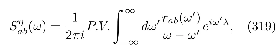
It is interesting to see that these functionswill be exactly canceled in these time evolution equations due to the following identity:

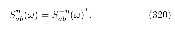
APPENDIX C:PROOF OF EQ.(193)

According to the definition,Eq.(41),the conjugation ofrab(ω)is

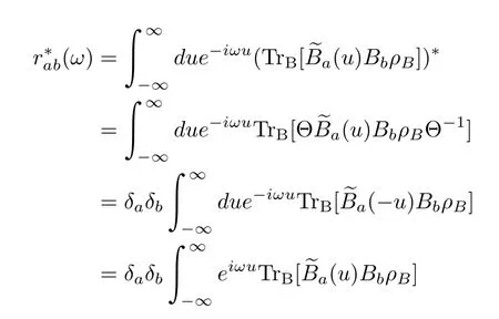
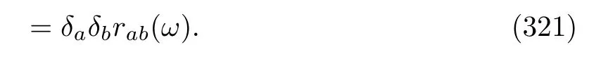
It was known early on that the matrix[rab(ω)]is Hermitian[78].Obviously,ifBaandBbare of different time-reversal types,rab(ω)is purely imaginary;otherwise,it is real.Using the same argument,we can also prove that

To illustrate Eq.(193),we present a simple example about a two-level system damped by a bath of harmonic oscillators[80,96].The total Hamiltonian is

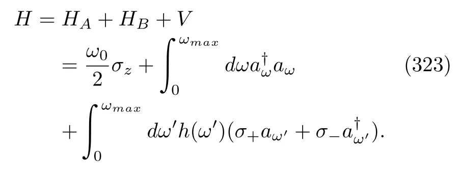
whereaω′is the continuous bosonic operator andω′is the frequency of each mode.The last integral term,the interactionV,can be rewritten as

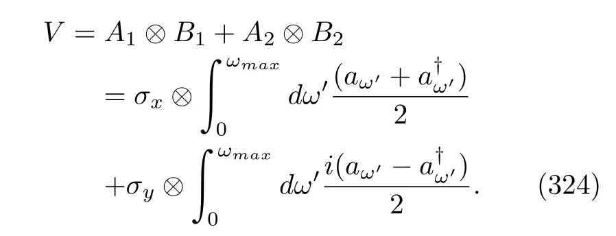
Obviously,the spectral decompositions ofA1andA2are

The reader is reminded that these Pauli matrices are not actual spin operators.Hence,the time reversals of theseAaandBa(a=1,2)operators are

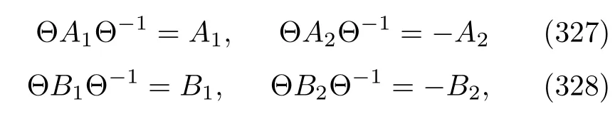
respectively. This also indicates that the interaction HamiltonianVis TRI.According to Eqs.(193)and(327),we can predict thatr11andr22are real and thatr12andr21are purely imaginary for the distinct Bohr frequencies−ω0andω0.One can verify this by explicitly calculating these coefficients:

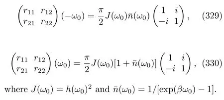
APPENDIX D:TIME REVERSAL IN THE MQMES

For the static and weakly driven Hamiltonian,the Bohr frequencyωis constant.According to our definition of backward processes,we easily see that the Bohr frequency and operatorsfor the backward process are the same as those of the forward process,namely,

On the other hand,according to the definition ofEq.(35),its time reversal is

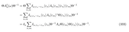
Considering that the HamiltonianHAis TRI and that its eigenvectors are non-degenerate[151],we have

Hence,the last equation is simply equal toIn other words,we proved Eqs.(194)and.(195)for the static and weakly driven Hamiltonian cases.

Now,let us check the adiabatically driven Hamiltonian case.Because the Hamiltonian of the backward process is Eq.(181),according to Eq.(65),the Bohr frequency and explicit expression of)are

respectively.This is because we have assumed that the HamiltonianHA(t)depends ontonly through the protocolsλ(t);see Eq.(80).Analogous to the static Hamiltonian case,according to the definition ofEq.(65),its time reversal is

The proof is obvious because it is completely analogous to Eq.(333);the additional time parameterthere does not affect the action of the time reversal.Hence,we confirmed the second equation,Eq.(195),for the adiabatically driven case.

The last case is about the periodically driven Hamiltonian(50).This is slightly involved because the Floquet basis(52)is time dependent.Wefirst note that the Hamiltonian of the backward process,

is also periodic,with the same periodicity Ω.Then,its Floquet basis can be constructed using the Floquet basis of the forward process:

The quasi-energy remains the same as that of the forward process,ϵn.Let us emphasize that these quasienergies are constant.The results can be directly con-firmed using the definition of the Floquet basis,E-q.(52).Because the Floquet basis is degenerate,we cannot expect that the RHS of Eq.(339)is simply|ϵn(t)〉,as in previous cases.Because the Bohr frequencyωis constant,we of course haveAccording to Eq.(57),the explicit expression of)is

where

The reader is reminded that the time parametersis present here because the Floquet basis is usually no longer only a function of the protocol,Now,we are in position to check Eq.(195)for periodically driven Hamiltonians.Recallingt+s=tf,we have

The multiplication of thefirst two terms after the Kronecker delta function is

To obtain the equation,we have performed a change of variablesu−tf→−uand used the periodic property of the Floquet basis.The integral term above is simply Eq.(341).Hence,we arrive at

APPENDIX E:EQUIVALENCE OF EQS.(231)AND(232)First,we write the deterministic part of Eq.(226)in the Schr¨odinger picture:

The density matrixσA(t)is obviously normalized,but the equation is non-linear.Noticing that its last sum term is simply the instantaneous total jump rate,E-q.(222),we suppose that

Inserting this into Eq.(345),we immediately obtain the linear evolution equation forπA(t),Eq.(234).On the other hand,if we substitute the above equation into Eq.(232),we have

On the other hand,in the case of the simple interaction Hamiltonian,Eq.(231)has the other expression if the system’s initial state is pure,e.g.,|ψ(0)〉〈ψ(0)|.Then,we have

whereU0(t,t′)is the effective time-evolution operator of the following equation:

namely,

The reader is reminded that|ϕ(t)〉is unnormalized.There are two ways to prove this equivalence.Thefirst way is to note that the propagatorG0,Eq.(235),and the time evolution operatorU0,Eq.(350)satisfy the following relation:

This structure is the same as that ofJ(ω),Eq.(233).Hence,Eq.(348)is an alternative expression of E-q.(232).Therefore,it is not strange that Eq.(231)is equal to Eq.(348).The other way is to note that the solution of the deterministic equation in Eq.(223)in the Schr¨odinger picture is related to the solution of Eq.(349)by

Substituting this result into Eq.(348),applying the same procedure as Eq.(347),and noting the definition in Eq.(221),we may directly prove the equivalence of Eqs.(231)and(348)without relying on Eq.(232).Let us again emphasize that Eq.(348)is valid only under the restrictions of a pure initial state of the system and a simple interaction Hamiltonian.

APPENDIX F:COMPUTATIONAL DETAILS OF THE PERIODICALLY DRIVEN TLS

For the reader’s convenience,we give some computational details about the TLS model.Although most of the details have been given in our previous paper[118],because we are concerned with the inclusive work here,some modifications are needed.

A.Directly simulating QJTs

Because the Floquet basis,Eq.(304),is complete and orthogonal,it shall be convenient to write operators and wave vectors in this time-dependent basis.For instance,theA(ω,t)operators in Eq.(306)are as follows:

The other three operatorsA(ω,t)withω=−ωL,−(ωL−Ω′),and−(ωL+ Ω′)are their adjoint operators.Note that to indicate that these Pauli matrices are not the conventional Pauli matrices,we add time parameters after these symbols.

According to our previous discussion,a QJT is a time evolution of a wave vector Ψ(t)in the Hilbert space of the TLS.This evolution is alternatively composed of a deterministic continuous evolution and stochastic jumps;see Eq.(223).Assuming that the continuous process starts from timetand ends at timet+τ,during this process,its deterministic equation is

0≤s≤τ.We expand the wave vector in the Floquet basis,that is,

Substituting this into Eq.(354),we obtain

where the coefficients are

respectively.Eqs.(356)have simple solutions:

Ψ(t+s)is not normalized. We denote the one Ψ(t+s),which isthesameasEq.(355)except thatµ±(s)therein are replaced byWe can determine the time durationτby solving the following equation:

whereη∈(0,1)is a uniform random number.

This smooth evolution is interrupted by a jump at timet+τ.The wave vector after the jump is

The probabilities of these jumps are proportional to

We list these six vectors in the following table:

Ψ′(t+τ) γ(ωL)(Ω/2Ω′)2 ħωL|u+(t+ τ)〉 (if µ−̸=0) r(ωL− Ω′)(‖µ−(τ)‖(δ− Ω′)/2Ω′)2 ħ(ωL− Ω′)|u−(t+ τ)〉 (if µ+̸=0) r(ωL+ Ω′)((‖µ+(τ)‖δ+ Ω′)/2Ω′)2 ħ(ωL+ Ω′)Ψ′(t+ τ) r(−ωL)(Ω/2Ω′)2 −ħωL|u−(t+ τ)〉 (if µ+̸=0) r(−(ωL− Ω′))(‖µ+(τ)‖(δ− Ω′)/2Ω′)2 −ħ(ωL− Ω′)|u+(t+ τ)〉 (if µ−̸=0) r(−(ωL+ Ω′))(‖µ−(τ)‖(δ+ Ω′)/2Ω′)2 −ħ(ωL+ Ω′)

where

After a vector is randomly chosen from the above,new rounds with continuous evolution and stochastic jump start until the end time is obtained.Finally,because we are concerned with the inclusive work,the initial wave vector is one of the energy eigenvectors forHA(0).

B.Solving Eq.(125)

In the Floquet basis,we may expand the HCOAas follows:

wherep±andpn,n=1,2,are the diagonal and nondiagonal elements of this density matrix in this basis,respectively.Substituting the expansion into Eq.(125)and doing simple algebra,we obtain the time-evolution equations for±(t)andpn:

Because we want to calculate the inclusive work CF,Eq.(129),the initial conditions areeiηHA(0)ρA(0)andρA(0)=e−βHA(0)/Z(0).Although these equations are a bit long and appear complicated,they are simply linear equations with constant coefficients.Hence,we can obtain their exact solutions.

[1]Mukamel S.Phys.Rev.Lett.,2003,90:170604

[2]Roeck W D,Maes C.Phys.Rev.E,2004,69:026115

[3]Roeck W D.C.R.Phys.,2007,8:674

[4]Esposito M,Harbola U,Mukamel S.Rev.Mod.Phys.,2009,81:1665

[5]Horowitz J M,Parrondo J M.New J.Phys.,2013,15:085028

[6]Esposito M,Mukamel S.Phys.Rev.E,2006,73:046129

[7]Crooks G E.Phys.Rev.A,2008,77:034101

[8]Talkner P,Campisi M,H¨anggi P.J.Stat.Mech.:Theor.Exp.,2009,P02025

[9]Suba¸si Y,Hu B L.Phys.Rev.E,2012,85:011112

[10]Horowitz J M.Phys.Rev.E,2012,85:031110

[11]Liu F.Phys.Rev.E,2012,86:010103

[12]Chetrite R,Mallick K.J.Stat.Phys.,2012,148:480

[13]Jaksic V,Pillet C A,Westrich M.J.Stat.Phys.,2013,154:153

[14]Hekking F W J,Pekola J P.Phys.Rev.Lett.,2013,111:093602

[15]Leggio B,Napoli A,Messina A,Breuer H P.Phys.Rev.A,2013,88:042111

[16]Liu F.Phys.Rev.E,2014,89:042122

[17]Liu F.Phys.Rev.E,2014,90:032121

[18]Silaev M,Heikkil¨a T T,Virtanen P.Phys.Rev.E,2014,90:022103

[19]Suomela S,Solinas P,Pekola J P,Ankerhold J,Ala-Nissila T.Phys.Rev.B,2014,90:094304

[20]Suomela S,Salmilehto J,Savenko I G,Ala-Nissila T,M¨ott¨onen M.Phys.Rev.E,2015,91:022126

[21]Suomela S,Kutvonen A,Ala-Nissila T.Phys.Rev.E,2016,93:062106

[22]Suomela S,Sampaio R,Ala-Nissila T.Phys.Rev.E,2016,94:032138

[23]Manzano G,Horowitz J M,Parrondo J M R.Phys.Rev.E,2015,92:032129

[24]Gasparinetti S,Solinas P,Braggio A,Sassetti M.New J.Phys.,2014,16:115001

[25]Cuetara G B,Engel A,Esposito M.New J.Phys.,2015,17:055002

[26]Alonso J J,Lutz E,Romito A.Phys.Rev.Lett.,2016,116:080403

[27]Gong Z.Ashida Y,Ueda M.Phys.Rev.A,2016,94:012107

[28]Strasberg P,Schaller G,Brandes T,Esposito M.Phys.Rev.X,2017,7:021003

[29]Pigeon S,Fusco L,Xuereb A,Chiara G D,Paternostro M.New J.Phys.,2015,18:013009

[30]Pigeon S,Xuereb A.J.Stat.Mech.:Theor.Exp.,2016,063203

[31]Garrahan J P,Lesanovsky I.Phys.Rev.Lett.,2010,104:160601

[32]Hickey J M,Genway S,Lesanovsky I,Garrahan J P.Phys.Rev.A,2012,86:063824

[33]˘Znidari˘c M.Phys.Rev.E,2014,89:042140

[34]Carrega M,Solinas P,Braggio A,Sassetti M,Weiss U.New J.,2015,17:045030

[35]Carrega M,Solinas P,Sassetti M,Weiss U.Phys.Rev.Lett.,2016,116:240403

[36]Manzano G,Galve F,Zambrini R,Parrondo J M R.Phys.Rev.E,2016,93:052120

[37]Schmidt R,Carusela M F,Pekola J P,Suomela S,Ankerhold J.Phys.Rev.B,2015,91:224303

[38]Chiara G D,Roncaglia A J.Paz J P.New.J.Phys.,2015,17:035004

[39]Wang C,Ren J,Cao J.Phys.Rev.A,2017,95:023610

[40]Blattmann R,Mølmer K.Phys.Rev.A,2017,96:012115

[41]Elouard C,Herrera-Mart´ı D A,Clusel M,Auff`eves A.npj Quantum Information,2017,3:9

[42]Perarnau-Llobet M,B¨aumer E,Hovhannisyan K V,Huber M,Acin A.Phys.Rev.Lett.,2017,118:070601

[43]Zhu L,Gong Z,Wu B,Quan H T.Phys.Rev.E,2016,93:062108

[44]Smith A,Lu Y,An S,Zhang X,Zhang J N,Gong Z,Quan H T,Jarzynski C,Kim K.New J.Phys.,2018,20:013008

[45]Gemmer J,Michel M,Mahler G.Lecture Notes in Physics,2005,29:53

[46]Boixo S,Rønnow T F,Isakov S V,Wang Z,Wecker D,Lidar D A,Martinis J M,Troyer M.Nat.Phys.,2014,10:218

[47]KosloffR.Entropy,2013,15:2100

[48]An S M,Zhang J N,Um M,Lv D S,Lu Y,Zhang J H,Yi Z Q,Quan H T,Kim K.Nat.Phys.,2015,11:193

[49]Rossnagel J,Dawkins S T,Tolazzi K N,Abah O,Lutz E,Schmidt-Kaler F,Singer K.Science,2016,352:325

[50]Bochkov G,Kuzovlev Y E.Zh.Eksp.Teor.Fiz,1977,72:238

[51]Evans D J,Cohen E G D,Morriss G P.Phys.Rev.Lett.,1993,71:2401

[52]Gallavotti G,Cohen E G D.Phys.Rev.Lett.,1995,74:2694

[53]Jarzynski C.Phys.Rev.Lett.,1997,78:2690

[54]Kurchan J.J.Phys.A:Math.Gen.,1998,31:3719

[55]Lebowitz J L,Spohn H.J.Stat.Phys.,1999,95:333

[56]Maes C.J.Stat.Phys.,1999,95:367

[57]Crooks G E.Phys.Rev.E,2000,61:2361

[58]Hatano T,Sasa S I.Phys.Rev.Lett.,2001,86:3463

[59]Seifert U.Phys.Rev.Lett.,2005,95:040602

[60]Kawai R,Parrondo J M R,VandenBroeck C.Phys.Rev.Lett.,98:080602

[61]Sagawa T,Ueda M.Phys.Rev.Lett.,2010,104:090602

[62]Degroot S R,Mazur P.Non-Equilibrium Thermodynamics,Dover,New York,1984

[63]Zubarev D.Nonequilibrium Statistical Thermodynamics,Plenum,New York,1974

[64]Kubo M T H N.Statistical Physics II:Nonequilibrium Statistical Mechanics,Springer,Berlin,1991

[65]Kurchan J.arXiv preprint cond-mat/0007360,2000

[66]Tasaki H.arXiv preprint cond-mat/0009244,2000

[67]Yukawa S.J.Phys.Soc.Jpn.,2000,69:2367

[68]Allahverdyan A E,Nieuwenhuizen T M.Phys.Rev.E,2005,71:066102

[69]Talkner P,Lutz E,H¨anggi P.Phys.Rev.E,2007,75:050102

[70]Andrieux D,Gaspard P.Phys.Rev.Lett.,2008,100:230404

[71]Campisi M,H¨anggi P,Talkner P.Rev.Mod.Phys.,2011,83:771

[72]Batalhao T B,Souza A M,Mazzola L,Auccaise R,Sarthour R S,Oliveira I S,Goold J,De Chiara G,Paternostro M,Serra R M.Phys.Rev.Lett.,2014,113:140601

[73]Jarzynski C,Quan H,Rahav S.Phys.Rev.X,2015,5:031038

[74]˘Znidari˘c M.Phys.Rev.Lett.,2014,112:040602

[75]Davies E B.Comm.Math.Phys.,1974,39:91

[76]Lindblad G.Comm.Math.Phys.,1976,48:119

[77]Gorini V,Kossakowski A,Sudarshan E C G.J.Math.Phys.,1976,17:821

[78]Breuer H P,Petruccione F.The theory of open quantum systems,Oxford university press,New York,2002

[79]Alicki B R,Lendi K.Quantum Dynamical Semigroups and Applications,Springer,Berlin,2010

[80]Rivas A,Huelga S F.Open Quantum Systems,Springer,Berlin Heidelberg,2012

[81]Spohn H,Lebowitz J L.Adv.Chem.Phys.,1978,39:109

[82]Spohn H.J.Math.Phys.,1978,19:1227

[83]Davies E B,Spohn H.J.Stat.Phys.,1978,19:511

[84]Alicki R.J.Phys.A:Math.Theor.,1979,12:L103

[85]Kohn W.J.Stat.Phy,2001,103:417

[86]Boukobza E,Tannor D J.Phys.Rev.A,2006,74:063823

[87]Alicki R.arXiv:1706.10257,2017

[88]Jarzynski C.Phys.Rev.E,1997,56:5018

[89]Seifert U.“Stochastic thermodynamics:An introduction”in Nonequilibrium Statistical Physics Today:Granada Seminar on Computational&Statistical Physics,AIP,2011,pp.56–76

[90]Teich W G,Mahler G.Phys.Rev.A,1992,45:3300

[91]Wiseman H,Milburn G.Phys.Rev.A,1993,47:1652

[92]Roeck W D,Maes C.Rev.Math.Phys.,2006,18:619

[93]Derezi´nski J,De Roeck W,Maes C.J.Stat.Phys.,2008,131:341

[94]Srinivas M,Davies E.Opt.Acta.,1981,28:981

[95]Plenio M,Knight P.Rev.Mod.Phys.,1998,70:101

[96]Carmichael H.An open systems approach to Quantum Optics:lectures presented at the Universit´e Libre deBruxelles,Springer,Berlin,1993

[97]Gardiner C,Zoller P.Quantum noise:a handbook of Markovian and non-Markovian quantum stochastic methods with applications to quantum optics,Vol.56,Springer,2004

[98]Wiseman H M,Milburn G J.Quantum measurement and control,Cambridge University Press,Cambridge,2010

[99]Ueda M.Phys.Rev.A,1990,41:3875

[100]Breuer H P.Phys.Rev.A,2003,68:032105

[101]Crooks G E,J.Stat.Mech.:Theory and Experiment,2008,P10023

[102]Bl¨umel R,Buchleitner A,Graham R,Sirko L,Smilansky U,Walther H.Phys.Rev.A,1991,44:4521

[103]Kohler S,Dittrich T,H¨anggi P.Phys.Rev.E,1997,55:300

[104]Breuer H P,Petruccione F.Phys.Rev.A,1997,55:3101

[105]Szczygielski K,Gelbwaser-Klimovsky D,Alicki R.Phys.Rev.E,2013,87:012120

[106]Garrahan J P,Armour A D,Lesanovsky I.Phys.Rev.E,2011,84:021115

[107]Hickey J M.Flindt C,Garrahan J P.Phys.Rev.E,2013,88:012119

[108]Lesanovsky I,van Horssen M,Gut˘a M,Garrahan J P.Phys.Rev.Lett.,2013,110:150401

[109]Touchette H.Phys.Rep.,2008,478:1

[110]Mollow B R.Phys.Rev.A,1975,12:1919

[111]Zoller P,Marte M,Walls D F.Phys.Rev.A,1987,35:198

[112]Horowitz J M,Sagawa T.J.Stat.Phys.,2014,156:55

[113]Esposito M,Van den Broeck C.Phys.Rev.Lett.,2010,104:090601

[114]Jarzynski C.C.R.Phys.,2007,8:495

[115]Campisi M,Talkner P,H¨anggi P.Phil.Trans.R.Soc.A,2011,369:291

[116]Imparato A,Peliti L.Phys.Rev.E,2015,72:046114

[117]Imparato A,Peliti L.Comptes Rendus Physique,2007,8:556

[118]Liu F.Phys.Rev.E,2016,93:012127

[119]Liu F,Xi J.Phys.Rev.E,2016,94:062133

[120]Pekola J P,Solinas P,Shnirman A,Averin D V.New J.Phys.,2013,15:115006

[121]Davies E B.Commu.Math.Phys.,1969,15:277

[122]Vinjanampathy S,Anders J.Contemp.Phys.,2016,57:545

[123]Pigeon S,Fusco L,Xuereb A,Chiara G D,Paternostro M.New J.Phys.,2015,18:013009

[124]Alicki R,Lidar D A,Zanardi P.Phys.Rev.A,2006,73:052311

[125]Gardiner C W.Handbook of Stochastic Methods,Springer,Berlin Heidelberg,1983

[126]Lindblad G.Comm.Math.Phys.,1975,40:147

[127]Schaller G.Open Quantum Systems Far from Equilibrium,Springer,Berlin,2014

[128]Geva E,KosloffR.Phys.Rev.E,1994,49:3903

[129]Albash T,Boixo S,Lidar D A,Zanardi P.New J.Phys.,2012,14:123016

[130]Nakajima S.Prog.Theor.Phys.,1958,20:948

[131]Zwanzig R.J.Chem.Phys.,1960,33:1338

[132]Kubo R.J.Phys.Soc.Jap.,1957,12:570

[133]Martin P C,Schwinger J.Phys.Rev.,1959,115:1342

[134]Grifoni M,Hnggi P.Phys.Rep.,1998,304:229

[135]Breuer H P,Huber W,Petruccione F.Phys.Rev.E,2000,61:4883

[136]Langemeyer M,Holthaus M.Phys.Rev.E,2014,89:012101

[137]Shirley J H.Phys.Rev.,1965,138:B979

[138]Zeldovich Y B.Sov.Phys.JETP,1967,24:1006

[139]Sambe H.Phys.Rev.A,1973,7:2203

[140]Breuer H P.Phys.Rev.A,2004,70:012106

[141]Amin M H S,Love P J,Truncik C J S.Phys.Rev.Lett.,2008,100:060503

[142]Messiah A.Quantum Mechanics,Vol.2,North-Holland,Amsterdam,1962

[143]Thunstr¨om P,˚Aberg J,Sj¨oqvist E.Phys.Rev.A,2005,72:022328

[144]Oreshkov O,Calsamiglia J.Phys.Rev.Lett.,2010,105:050503

[145]Risken H H.The Fokker-Planck equation:methods of solution and applications,Springer-Verlag,Berlin,1984

[146]Ballentine L E.Quantum mechanics:a modern development,World Scientific,Singapore,2014

[147]Bochkov G,Kuzovlev Y E.Physica A,106:1981,443

[148]Hummer G,Szabo A.Proc.Natl.Acad.Sci.U.S.A.,2001,98:3658

[149]Polkovnikov A.Ann.Phys.,2010,325:1790

[150]Kac M.Trans.Am.Math.Soc.,1949,65:1

[151]Sakurai J J.Modern Quantum Mechanics,Addison Wesley,California,1994

[152]Quan H T,Jarzynski C.Phys.Rev.E,2012,85:031102

[153]Esposito M,Harbola U,Mukamel S.Rev.Mod.Phys.,2014,86:1125

[154]Liu F,Ouyang Z C.Chin.Phys.B,2014,23:070512

[155]Pusz W,Woronowicz S L.Comm.Math.Phys.,1978,58:273

[156]Agarwal G S.Z.Physk.,1973,258:409

[157]Alicki R.Rep.Math.Phy.,1976,10:249

[158]Andrzej Kossakowski V G.Frigerio A,Verri M.Comm.Math.Phys.,1978,60:96

[159]Ciliberto S.Phys.Rev.X,2017,7:021051

[160]Kelley P L,Kleiner W H.Phys.Rev.,1964,136:A316

[161]Mollow B R.Phys.Rev.,1968,168:1896

[162]Carmichael H J,Singh S,Vyas R,Rice P R.Phys.Rev.A,1989,39:1200

[163]Nagourney W,Sandberg J,Dehmelt H.Phys.Rev.Lett.,1986,56:2797

[164]Sauter T,Neuhauser W,Blatt R,Toschek P E.Phys.Rev.Lett.,1986,57:1696

[165]Bergquist J C,Hulet R G,Itano W M,Wineland D J.Phys.Rev.Lett.,1986,57:1699

[166]Basch´e T,Kummer S,Br¨auchle C.Nature,1995,373:132

[167]Peil S,Gabrielse G.Phys.Rev.Lett.,1999,83:1287

[168]Gleyzes S,Kuhr S,Guerlin C,Bernu J,Del´eglise S,HoffU B,Brune M,Raimond J M,Haroche S.Nature,2007,446:297

[169]Murch K,Weber S,Macklin C,Siddiqi I.Nature,2013,502:211

[170]Sun L,Petrenko A,Leghtas Z,Vlastakis B,Kirchmair G,Sliwa K M,Narla A,Hatridge M,Shankar S,BlumoffJ.Nature,2013,511:444

[171]Vool U,Pop I M,Sliwa K,Abdo B,Wang W,Brech

t T,Gao Y Y,Shankar S,Hatridge M,Catelani G,Mirrahimi M,Frunzio R G L D M,Schoelkopf L.Phys.Rev.Lett.,2014,113:247001

[172]Campagne-Ibarcq P,Six P,Bretheau L,Sarlette A,Mirrahimi M,Rouchon P,Huard B.Phys.Rev.X,2016,6:011002

[173]Mølmer K,Castin Y,Dalibard J.J.Opt.Soc.Am.B,1993,10:524

[174]Barchielli A,Gregoratti M.Quantum Trajectories and Measurements in Continuous Time,Springer,Berlin Heidelberg,2009

[175]Parthasarathy K.An Introduction to Quantum S-tochastic Calculus,Springer,Basel,1992

[176]Kist T B L,Orszag M,Brun T A,Davidovich L.J.Opt.B:Quantum Semiclass.Opt.,1999,1:251

[177]Brun T A.Am.J.Phys,2001,70:719

[178]Attal S,Pautrat Y.Annales Henri Poincar`e,2006,7:59

[179]Braginsky V B,Khalili F Y,Thorne K S.Quantum Measurement,Cambridge University Press,Cambridge,1992

[180]Breuer H P,Petruccione F.Phys.Rev.E,1995,52:428

[181]Horowitz J M,Vaikuntanathan S.Phys.Rev.E,2010,82:061120

[182]Hush M R,Lesanovsky I,Garrahan J P.Phy.Rev.A,2015,91:032113

[183]de Vega I,Alonso D.Rev.Mod.Phys..2017,89:015001

[184]Daley A J.Adv.Phys,2014,63:77

[185]Stroock D W,Varadhan S S.Multidimensional Diffusion Processes,Springer,Berlin,2005

[186]Majumdar S N.Current Science,2005,89:2076

[187]Schlosshauer M A.Decoherence and the quantum-toclassical transition,Springer,Berlin Heidelberg,2007

[188]Wang Q,Quan H T.Phys.Rev.E,2017,95:032113