Numerical studies of static aeroelastic effects on grid fin aerodynamic performances

Chengde HUANG,Wen LIU,Guowei YANG,*

aInstitute of Mechanics,Chinese Academy of Sciences,Beijing 100190,China

bSchool of Engineering Science,University of Chinese Academy of Sciences,Beijing 100049,China

Numerical studies of static aeroelastic effects on grid fin aerodynamic performances

Chengde HUANGa,b,Wen LIUa,Guowei YANGa,b,*

aInstitute of Mechanics,Chinese Academy of Sciences,Beijing 100190,China

bSchool of Engineering Science,University of Chinese Academy of Sciences,Beijing 100049,China

The grid fin is an unconventional control surface used on missiles and rockets.Although aerodynamics of grid fin has been studied by many researchers,few considers the aeroelastic effects.In this paper,the static aeroelastic simulations are performed by the coupled viscous computational fluid dynamics with structural flexibility method in transonic and supersonic regimes.The developed coupling strategy including fluid–structure interpolation and volume mesh motion schemes is based on radial basis functions.Results are presented for a vertical and a horizontal grid fin mounted on a body.Horizontal fin results show that the deformed fin is swept backward and the axial force is increased.The deformations also induce the movement of center of pressure,causing the reduction and reversal in hinge moment for the transonic flow and the supersonic flow,respectively.For the vertical fin,the local effective incidences are increased due to the deformations so that the deformed normal force is greater than the original one.At high angles of attack,both the deformed and original normal forces experience a sudden reduction due to the interference of leeward separated vortices on the fin.Additionally,the increment in axial force is shown to correlate strongly with the increment in the square of normal force.

©2017 Chinese Society of Aeronautics and Astronautics.Production and hosting by Elsevier Ltd.This is anopenaccessarticleundertheCCBY-NC-NDlicense(http://creativecommons.org/licenses/by-nc-nd/4.0/).

1.Introduction

The grid fin,also called the lattice fin,is an unconventional lifting and control surface consisting of a grid structure supported by the outer frame,and has been used on missiles and rockets due to its higher aerodynamic performances than conventional planar control surfaces.

Previous investigations suggest that the use of grid fins has several advantages.1The grid fins have better stall characteristics due to the increased normal forces over a wider range of angles of attack,which improves the control efficiency of grid fins at high angles of attack compared to the planar control surfaces.Because of the use of short chord,the grid fins usually produce small hinge moments and can reduce the required power of the actuator system.Besides,the unique internal constraints of the grid fins help to improve the structural strengthto-weight ratio.

Aerodynamic characteristics of grid fins have been studied experimentally by many researchers.Wind tunnel tests showed that the shape of the outer frame and the internal web thickness have great effects on the drag characteristics but have slight impacts on the fin normal forces.2Curved grid fins are helpful for compact packaging against the rocket bodies and the curvature effects on aerodynamic characteristics were shown to be limited.3The sweep back effects were also investigated,indicating that the drag forces can be increased by the sweep back angle.3Experiments with deflected grid fins installed on a projectile body were performed in wind tunnels4,and the test results showed that the fin deflection angles affected the aerodynamic coefficients significantly and the roll moment reversal was observed at large deflection angles in a subsonic condition.

Numerical simulations were also performed to predict the aerodynamics of the grid fins.For example,vortex lattice method and shock-expansion theory were used in the aerodynamic calculations in subsonic and supersonic flows,respectively,while the nonlinear effects of leeward separated vortices at high angles of attack were considered by the empirical relations.5,6Recently,high-fidelity computational fluid dynamics(CFD)techniques were used to solve the flow fields around the grid fins with high accuracy.The aerodynamic simulations of a body and grid fin combination were performed using the unstructured-mesh solver(FLUENT).7,8Detailed pressure distributions were computed,which reveals the complicated flow structures near the grid fins.In transonic conditions,the flows passing through grid fins are choked within the cells and the development of choking was investigated using CFD techniques.9The transonic choked flow causes the maximum of drag coefficient,to reduce which,the sweptback grid fin with sharp leading edges was designed and CFD computations proved this new configuration conduces to alleviating the flow choking and the associated drag.10Despeyroux et al.11used the unstructured finite volume based code SU2 to analyze the static and dynamic flight stabilities of gird fin controlled missiles.The pitching motions were simulated by rigid motions of the computational domain and the results indicated that the missile was statically unstable at moderate angles of attack in a transonic condition due to the choking effect,but dynamically stable in both transonic and supersonic conditions.

Unlike conventional planar control surfaces,grid fins are installed perpendicularly to the incoming flow and the unique cell structures enlarge the windward area and increase the axial forces,which have a potential of pushing the grid fins backward.In the previous studies,the grid fins were assumed to be rigid and therefore no fluid–structure interaction need to be considered in the CFD simulations.However,because the actual fin structures are elastic,the grid fins under aerodynamic loads could be deformed and then the deformations in return interact with the fluid field and cause the redistributions of aerodynamic loads.This aeroelastic effect can be considerably strong due to the specific geometric structure of the grid fins and may change their aerodynamic performances significantly.In the past decades,numerical solutions of aeroelastic computations have been attempted for the analyses of wings and aircraft.Mian et al.12coupled the finite element method and Reynolds-averaged Navier–Stokes solver to compute the static deformations of a flexible wing using the radial basis function method for fluid–structure interpolations and CFD mesh motions.Bartels et al.13computed the transonic flutter boundary of an aircraft model using the Navier–Stokes code FUN3D for unsteady aerodynamic simulations and the modal technique to solve structural equations of motion.Lamorte and Friedmann14developed a framework of hypersonic aerothermoelastic analysis.The CFD++code was used to compute aerodynamic loads and heat-flux,coupled with the structural heat and dynamics analyses using the finite element method code MSC.NASTRAN.

As far as we know,the grid fin aeroelasticity was seldom studied before,so it is necessary to construct the numerical strategy for the fluid–structure interaction analyses and to investigate the aeroelastic effects on grid fin aerodynamic performances.

In this paper, the computational fluid dynamicscomputational structural dynamics(CFD-CSD)coupling method is used in the aeroelastic simulations which decouples the fluid–structure interaction problems and solves the aerodynamic forces and structural motions separately.The forces and displacements between the fluid and structure domains are communicated at the interface using interpolation techniques.Because of the complicated geometry of the grid fins,it is quite challenging to implement a proper interpolation scheme that meets the accuracy and efficiency requirements.In the current study,the time efficient fluid–structure interpolation and mesh motion schemes based on radial basis functions(RBF)are developed for the static aeroelastic simulations and it can be demonstrated that the developed scheme is effective for such complicated geometries as the grid fins.The organization of the paper is as follows.Section 2 describes the numerical strategy for the aeroelastic simulations of the grid fins.The simulation results and discussions are presented in Section 3,followed by the conclusions in Section 4.

2.Numerical approach

2.1.Model descriptions

2.1.1.Geometry model

The geometric model evaluated in the present study originates from the experimental model tested by Miller and Washington.2The model shown in Fig.1(a)is 52 in(1 in=25.4 mm)long,with a 15 in tangent ogive nose,and the diameter of the body is 5 in.There are four fins mounted 2 calibers ahead of the base.The right-handed coordinate system is located at the nose of the body,withxaxis pointing downstream along the center line,yaxis upward andzaxis along the left side viewed from the rear.The outer frame thickness of the grid fin tested in the experimental model varies from 0.02 into 0.06 in.For computational convenience,the outer frame thickness was simplified as a constant of 0.04 in by Lin et al.15,while the total windward area of grid fin remained the same as the experimental model.The simplified model is adopted in the present paper with rectangular outer frame shape.In addition,the thickness of the internal web is 0.008 in and the chord length of grid fin is 0.384 in.

2.1.2.CFD mesh

The CFD model was designed for the aerodynamic simulations of the grid fins.The hybrid mesh was generated with clustered boundary layer cells,and the total number of volume cells is about 14 million.There are 0.63 million trilateral elements generated on the surface(Fig.1(a)),while the grid refinement is performed with about 0.15 million cells on each fin surface(Fig.1(b)).The whole computational domain is a regular hexahedron with approximately 10 times body length in thexdirection and about 40 times diameter length in theyandzdirections,respectively.

2.1.3.Structural model

A three dimensional structural model was constructed for the grid fin,based on which the finite element method can be utilized to calculate the structural responses of the model under the aerodynamic loads.The solid elements are used to discretize the grid fin shown in Fig.2(a)and(b)plots the detailed mesh distributions near the foot.The outer frame and the internal webs are meshed using 8-node hexahedrons except for their junctions at which 6-node wedges are used.The structural model has 2620 elements in total including 2580 hexahedrons and 40 wedges,which is constructed by 5760 nodes.A typical metallic material,the copper with elastic modulus 110 GPa,Poisson’s ratio 0.31,is used for the material property of the grid fin.It should be noted that the body was not included in the structural model in the current study,since the body is much stiffer than the grid fins and hence was assumed to be rigid to simplify the aeroelastic problem.

In an actual flight,the grid fins are connected to the actuators which control the packaging,deployments and deflections of the fins,hence there exists inevitable joint stiffness at the connections.It is not necessary to build a detailed finite element model for the connection structure since our focus is on the grid fin.Instead,a spring element is designed to model the joint stiffness effect.In the present paper,the spring element is added at the root of the grid fin though it is not included in the original test model,and its location is(41.808,0,2.559)inch for the left fin shown in Fig.2(a).The hinge line coincides with the axis of symmetry along thez-axis direction.Two degrees offreedom are released at the spring element.The rotation around the hinge line is defined as the twist,while the rotation about another line along theyaxis direction(Fig.2(a))is defined as the bending.The stiffness coefficients are designed to be 50 N·m/rad in the bending direction and 25 N·m/rad in the twist direction,respectively.Additionally,the multiple-point-constraint(MPC)16is used to connect the spring element and the solid elements at the root.This structural model was tested using the general purpose finite element analysis program MSC.NASTRAN and the flexibility matrix of the grid fin was computed for the aeroelastic analyses which will be described in the next section.

2.2.Fluid-structure interaction techniques

2.2.1.Strategy for static aeroelastic analysis

The solution strategies of the coupled fluid–structure system are classified into two categories17:the monolithic approach that solves the aerodynamic forces and structural motions simultaneously using the integrated aero-structure solver but causes additional complexities;and the partitioned approach that solves the aerodynamic forces and the structure motions in a separate manner with additional data communications between different solvers.In the current study,the static aeroelastic problem is solved using the partitioned approach which allows the use of the existing CFD solvers and structural analysis tools.

Static aeroelasticity studies the interactions between the static structural deformations and the aerodynamic loads.The elastic structure may deform under the aerodynamic forces generated by the fluid flows,while the deformations of the structure can alter the surrounding flows and change the aerodynamic loads in response,until the static equilibrium is obtained.To achieve this state numerically,an iterative process is performed as follows:

(1)Compute the aerodynamic loads using CFD.

(2)Interpolate the forces from aerodynamic nodes onto structural nodes.

(3)Calculate the structural displacements using the flexibility method.

(4)Interpolate the displacements from structural nodes onto aerodynamic nodes at the interface and deform the volume mesh.

(5)Repeat(1)to(4)until the static equilibrium is achieved.

2.2.2.Flexibility method

The flexibility method is adopted to calculate the structural displacements so that the elastic behavior of grid fins can be analyzed under the aerodynamic loads.The flexibility matrix C was achieved in advance by linear static analyses using MSC.NASTRAN,therefore the structural displacements u can be computed by

where F denotes the vector offorces acting on the structural nodes.This method is based on the linear assumption and is suitable for small deformation problems,e.g.grid fins.The matrix size of C is 3N×3N,whereNdenotes the number of structural nodes.Since only simple matrix multiplications are required,the flexibility method can be integrated with CFD codes for fluid–structure interaction analyses without much work.

2.2.3.Fluid-structure interpolation

The partitioned approach decouples the fluid–structure interaction problem,and solves the aerodynamic forces and structural motions separately.Because of the independent manners of the aerodynamic and structural models,the aerodynamic nodes are usually inconsistent with the structural nodes at the interface.Therefore interpolations need to be implemented to transfer forces and displacements between the aerodynamic and structural nodes following physical laws,including the conservation of total force,moment and energy.The interpolations with RBF are based on the spatial positions of control points only and can be performed on arbitrary point clouds with no connectivity information required.The general form of RBF interpolation is17

which is a three-dimensional extension from the infinite plate spline(IPS)method18and can be recognized as the equations of equilibrium.There are many radial basis functions17available and the most widely used functions include the Wendland’s C0 function

wheredis the support radius of the radial influence range and is chosen to be a suitable value to consider enough points near the interface and exclude the points far away.19In the current study,the support radius is 7.87 in which is about two times the grid fin height defined as the length from the root to the top.Comparisons of interpolation errors between the C0 and C2 functions of Wendland are performed later,and the better one is chosen for the aeroelastic simulations.The displacements and forces in all the three directions should be exchanged between the aerodynamic nodes and the structure nodes.Without loss of generality,the interpolation ofxcomponent is described below.Applying Eq.(2)to allNstructural nodes,with the combination of Eq.(3),yields

where subscript ‘s” denotes the structure nodes.The solution of Eq.(6)yields the coefficients λ,then the displacements of allMaerodynamic nodes on the surface can be attained by

where subscript ‘a” denotes the aerodynamic surface nodes.

Integrations of pressures and viscous stresses on the surface yield the vector offorces faat the aerodynamic nodes.For the interpolations of structural forces,the aerodynamic/structural coupling matrix needs to be calculated directly in Ref.17which requires costly computations.In this paper,a positive definite system of linear equations is constructed by the introduction of pseudo structural forcesThe acting forces fson the structural nodes then can be calculated more efficiently via the solution of the linear system,avoiding the costly computations of the aerodynamic/structural coupling matrix.The relation of equivalence of virtual work can be rewritten as

Substitution of Eq.(6)and Eq.(7)into Eq.(8),yields

then fscan be attained by solving the linear Eq.(9).The first four rows of Eq.(9)are

which suggest the conservation of total force and total moments when communicating the forces between the aerodynamic and the structural nodes.

2.2.4.Volume mesh deformation scheme

The deformation offluid–structure interface,due to the deflection of the structure,usually requires the updates of the volume mesh.It is tedious to regenerate the entire mesh manually especially in the case of aeroelastic simulations which require mesh update to be performed repeatedly.Mesh deformation is the preferred choice to update the CFD mesh automatically and various methods have been investigated,i.e.transfinite interpolation(TFI),20spring analogy(SA),21PDE solution method,22and Delaunay mapping,23etc.However,all the mesh type dependent methods require the knowledge of the grid connectivity.The displacements of interior grids usually need to be solved by a system of equations including all the points in the domain,and can therefore be computationally expensive.

In the present paper,the RBF method is used to deform the mesh.Similar to Eq.(2),the interpolation relation for the mesh motion is

where the linear terms are removed since the conservations of the total force and moments are not needed,andNsprefers to the number of control points driving the mesh motion and is usually less thanM,the total number of the aerodynamic surface nodes.Substituting theNspcontrol points into Eq.(11),yields

where ΔxaNspdenote the displacements ofNspcontrol points extracted from Δxa.The coefficients α1, α2,..., αNspare attained by the solution of Eq.(12),and then the substitutions ofvolume node coordinatesinto Eq.(11)yield the displacements,

where subscript ‘v” denotes the volume nodes,andNvpthe total number of volume nodes.Then,Δxvare superposed on the current coordinates to update the mesh.

The computational effort associated with the volume mesh updates scales withNvp×Nsp.Selecting allMsurface points as control points will make calculations expensive.To reduce the computational cost,Rendall and Allen24proposed the ‘greedy’algorithm to reduce the size of the control points,which sacrifices the accuracy of the deformation at the surface with an acceptable error.Different error signals related to the ‘greedy’algorithm were tested,and the comparisons of the interpolation errors showed that the unit function provided the smallest errors as well as the best efficiency.25Therefore,the error signal using the unit function is adopted for the selection of the reduced control points in this paper.

2.2.5.CFD solver

The unstructured finite volume-based solver Ansys Fluent 14.0 is used for the steady CFD simulation.The governing equations are three-dimensional compressible Navier–Stokes equations in the conservation form:

where W denotes the conservative variables,Ω the control volume,Sthe surface area,Fcthe vector of convective fluxes evaluated by the Roe-FDS scheme,Fvthe vector of viscous fluxes,and H the source terms which vanishes in the present calculations.The gradients are evaluated by the Green-Gauss scheme,while the turbulence is simulated using the one-equation Spalart–Allmaras model.The second-order upwind scheme is used for the spatial discretizations of the flow variables and the turbulent viscosity.

For aeroelastic simulations,the flexibility method,fluid–structure interpolation and mesh deformation schemes based on the RBF method were implemented into the CFD solver through the user-defined functions.26

3.Results and discussion

The results and discussion are divided into four parts: firstly,the study of RBF interpolation accuracy;secondly,the validations of the CFD simulations;thirdly,the static aeroelastic analyses of the left fin;and finally,the analyses of the upper fin.

3.1.Assessment of RBF accuracy

Because of the complex geometric topology of the grid fin,it is a challenge to meet the accuracy requirement when performing the interpolations and mesh motions.In this section,the interpolation precision is studied with the Wendland’s C0 and C2 functions,and the reduced set of control points is determined.

The first four structural mode shapes of the grid fin are used to examine the RBF interpolation errors for accuracy evaluation.The ‘greedy’algorithm is used to select the reduced set of control points,based on which the displacements at all surface points are interpolated.The errorsare the differences between the exact values and the interpolated values at pointiin thex,y,zdirections.These errors are further squared and normalized with the maximum displacementumaxto give the scalar error:

Fig.3 shows the mode shapes and their error distributions on the surface using the C2 function with 200 control points.The first mode denotes the bending deformation and the maximum interpolation error is the order of 10-3occurring at the lower part of the fin.The second mode denotes the deformation of twist about the hinge line with the maximum interpolation error of the order of 10-3.The third mode denotes the deformation in they-zplane and the maximum error reaches the order of 10-2.The fourth mode denotes the stretch along the symmetric axis and its maximum interpolation error is the order of 0.1 occurring at the center of the internal webs.It can be shown that the higher order the mode is,the more complicated the shape will be with larger interpolation errors.It is demonstrated later that under aerodynamic loads,the deformed grid fins are close to the combinations of low order mode shapes,which produce errors small enough.Hence,the RBF method is satisfactory for the aeroelastic simulations of grid fins.

Fig.4(a)and(b)compare the interpolation errors between the Wendland’s C0 and C2 functions.The errors are calculated as the maximum errorEmaxand the average errorEavg,respectively.Both theEmaxandEavgdecrease as the number of control points increases for all the mode shapes.The errors associated with the C2 function are shown to be consistently smaller than those with the C0 function.The comparison of the control points(Fig.5)shows that there are more points scattering inside the grid fin with more uniform global point distributions using the C2 function than using the C0 function,which induces larger errors on the internal cell walls(Fig.5(b)).Therefore,the Wendland’s C2 function performs better than the C0 function and is adopted in the present aeroelastic simulations.The number of the control points is designed to be 500,which not only ensures the interpolation errors small enough,but also saves much computation work for the mesh deformations.

3.2.Validations

The flow conditions are given in Table 1 including the subsonic(Ma=0.7),transonic(Ma=1.2)and supersonic(Ma=2.5)regimes.The aerodynamic and aeroelastic characteristics arestudied for both the upper and left fins in the present work,since the surrounding flow fields are different between the vertical and the horizontal grid fins at nonzero angles of attack.The reference length and the reference area are set to be equal to the diameter(5.0 in)and the body cross sectional area(19.635 in2),respectively.The sign conventions of the aerodynamic coefficients are shown in Fig.6,whereCLis the lift coefficient,CDis the drag coefficient,CAis the axial force coefficient,CNis the normal force coefficient,CHMis the hinge moment coefficient,V∞is the freestream velocity,α is the angle of attack.

Table 1 Free-stream conditions.

To validate the CFD mesh and the numerical results,the computed force and moment coefficients are compared with the experiment results at angles of attack ranging from-5°to 15°(Fig.7).Since the wind tunnel test data are only available for the horizontal fin in the Ref.2,the validations of the CFD simulations are only performed for the left fin.

The normal force coefficientsCNbecome higher as the angle of attack increases,and the slopes of the linear portions ranging from-5°to 5°are in a quite good agreement between the computed results and the experimental results(Fig.7(a)–(c)).The nonlinear characteristics of normal forces at higher angles of attack are well predicted with reasonable errors.The result deviations between the computations and measurements at high incidences are within 6%at Mach number 0.7,11%at Mach number 1.2 and 12%at Mach number 2.5,respectively.

The axial force coefficientsCAare computed accurately with errors less than 5%at Mach number 1.2 and Mach number 2.5.The computed axial force coefficients at zero angle of attack are 0.0479 for Mach number 0.7,0.0586 for Mach number 1.2,0.0523 for Mach number 2.5 respectively,which suggests that the highest drag exists at the transonic condition.Fig.7(d)shows the hinge moment coefficientsCHMversus angles of attack at Mach number 0.7 and Mach number 2.5,and the different curve trends are predicted well.The hinge moment coefficients at Mach number 2.5 are much smaller than those at Mach number 0.7.This is because the chordwise center of pressure at Mach number 2.5(near mid-chord)is closer to the hinge line than that at Mach number 0.7(near 25%chord).2Therefore,the moment arm and moment coefficient about the hinge line at Mach number 2.5 are smaller than those at Mach number 0.7.

3.3.Static aeroelastic analyses of left fin

3.3.1.Convergence

To achieve the static equilibrium state of the grid fin,the iterative process described in Section 2 is performed.The maximum displacementumaxis normalized with the grid fin chord lengthc=0.384 in.The final equilibrium state is defined as the increment ofumax/creduces to the order of 10-4.Fig.8(a)and(b)shows the convergence histories at α =5°in the transonic condition,which is defined in Table 1.The converged result is obtained within 5 iterative steps.

3.3.2.Static aeroelastic effects

The effects on aerodynamic performances of the left fin are studied in this subsection.The results at-5°to 15°angles of attack are shown from Figs.9–14,where ’rigid’denotes the original state and ’elastic’denotes the deformed state.The discussions are as follows.

(1)Deformation and normal force

The top view of the deformed fin relative to the original fin at α =10°at Mach number 1.2 is illustrated with Fig.9.Under aerodynamic loads,the deformations of the left fin mainly contain three parts,the bending,the elastic twist,and the movement in they-zplane.It is noted that the bending plays a major part in the deformations.What’s more,the elastic twist is induced by the hinge moment and tends to increase the effective angle of attack of the left fin.The change in incidence can be illustrated with the change in pressure distribution.Fig.11(a)shows the pressure coefficientCpcontours on the rigid fin at α =10°,and the blue contours on the webs and outer frame indicate the suction regions contributing to the normal force.As for the elasticCp(Fig.11(b)),there are larger suction areas compared with the rigid case,so that the normal force is increased slightly at Mach number 1.2(Fig.10(a)).

At Mach number 2.5,the change inCNis shown to be insignificant(Fig.10(b)).This is because in this Mach regime,the elastic twist angle is tiny due to the small hinge moment,so that the effective angle of attack is nearly unchanged.

(2)Axial force

The elasticCAis about 10%and 4%larger than the rigidCAfor Mach number 1.2 and Mach number 2.5,respectively(Fig.12(a)).The reason is the sweep back effect caused by bending deformation.In Ref.3,the grid fin was rigid but could be deployed and swept backward by controls.The angle between the original fin and the swept fin was investigated experimentally and the results showed that the sweep back angle was to augment the drag significantly.In the current study,when the left fin produces bending deformations,it is also swept backward and the windward area increases,thus the axial force coefficients are increased.

(3)Hinge moment

At Mach number 1.2,the rigidCHMis generally larger than elasticCHM(Fig.13(a)).The difference between the elastic and rigidCHMis mainly due to the movement of center of pressure.The position of chordwise center of pressurexCPcan be calculated as

wherexHdenotes thexcoordinate of the hinge line,Lthe reference length.The(xH-xCP)/cvalues are summarized in Table 2.In the transonic condition,the center of pressure is between 20%and 30%of the grid fin chord.When the elastic cases are considered,(xH-xCP)/cis reduced,indicating the center of pressure shifts backward.As a result,the moment arm for the normal force about the hinge line is reduced,so that the elasticCHMis generated smaller than the rigid one.

However,at Mach number 2.5,when α＞0°,the rigidCHMis positive but the elasticCHMis negative,indicating that the reversal in hinge moment occurs(Fig.13(b)).In this supersonic flow,the center of pressure is very near the mid-chord for the rigid cases,so that it will move behind the hinge line when the fin is deformed(Table 2).Therefore,the elastic normal forces generate negative hinge moments.

(4)Normalized maximum displacement

At Mach number 1.2,theumax/creaches the minimum at α =0°and then increases rapidly until α =10°(Fig.14(a)),while the low growth rate at α =15°may be due to the slight decrease in elasticCA.However,the curve trend observed at Mach number 2.5 is different from that observed at Mach number 1.2.Theumax/cgets the maximum at α =0°and then declines in this supersonic flow(Fig.14(b)).This curve trend is similar to that of elasticCA(Fig.12(b)).

3.4.Static aeroelastic analyses of upper fin

3.4.1.Changes in flow field in transonic condition

At Mach number 1.2,the static aeroelasticity of the upper fin is studied.Because both the flow field and the deformed configuration are symmetric,it is convenient to analyze the aeroelastic effects by visualizations of flow field on the symmetry plane(z=0).This symmetry plane cuts the upper fin and there are four internal spars,the top and the bottom spars in figures.As shown in Fig.15(a)for the rigid Mach contours at α =0°,a bow shock wave is formed in front of the fin and reduces the speed of flow to subsonic value.The flow passing through the cells accelerates so that the sonic condition is met near exits,indicating the flow-choking phenomenon occurs.What’s more,the supersonic regions on the internal spars are much like the flow field around a transonic airfoil.Fig.15(b)shows the deformed Mach contours,and the supersonic regions become larger than those in the rigid case within the cells.

The rigidCpcontours(Fig.16(a))show that there are suction regions on the upper surfaces of the internal spars so that the normal force points upward.The reason is that streamlines are deflected after the bow shock and the upward component of velocity is created in front of the fin,so that the effective angle of attack is actually positive at α =0°.The deformedCpcontours(Fig.16(b))illustrate that the suction areas contributing to the normal force grow so that the elasticCN(0.0386)is larger than the rigidCN(0.0173),confirming that the aerodynamic changes for the elastic grid fin mainly come from the increased local effective angle of attack due to the structural deformations.

3.4.2.Changes in flow field in supersonic condition

For the case of Mach number 2.5,Fig.17 shows the pressure contours on thez=0 cutting plane at three angles of attack.

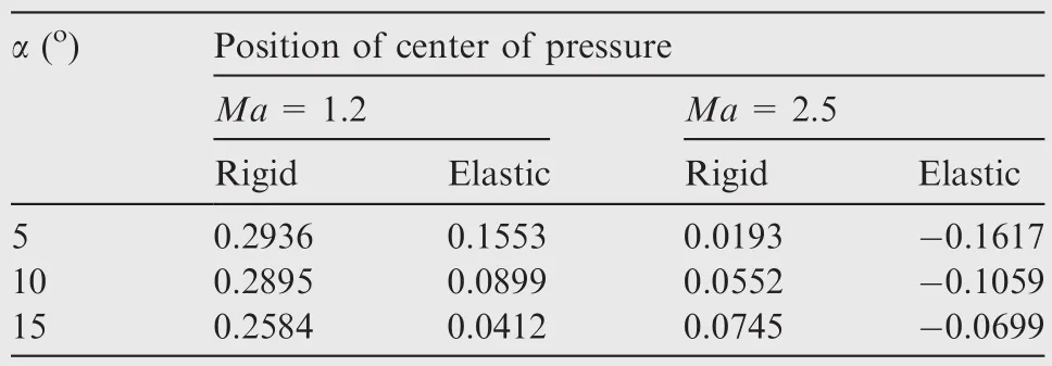
Table 2 Position of center of pressure.

The cutting sections are rectangular.In this supersonic regime,the bow shock wave in front of the fin has been swallowed,and the flow choking has vanished within the cells.However,each spar acts like a supersonic thin wing,with a detached bow shock formed about the blunt leading edge.The flow is compressed across the shock,followed by an expansion fan emanating from the corner of the leading edge.The shock and expansion waves intersect with the others coming off the opposite side within each cell,and then continue propagating downstream,leading to more intersections behind the grid fin.For the rigid case at α =0°(Fig.17(a)),the pressure distributions are almost the same between the upper and lower surfaces of each internal spar,so that the rigid normal force coefficient is near zero.As for the elastic case(Fig.17(d)),the expansion of flow on the upper surface becomes more intense than that on the lower surface,indicating the local angle of attack of each internal spar is increased.Therefore,the elasticCN(0.0256)is larger than the rigidCN(0.002)at α =0°.

3.4.3.Linear and nonlinear characteristics of elastic normal force

At Mach number 1.2,the normal force coefficients at angles of attack from-14°to 18°are illustrated with Fig.18(a).The elasticCNis generally greater than the rigidCNbecause of the increased effective angle of attack.When the body is at angle of attack from-14°to 0°,indicating the upper fin is in the windward side,the curve of elasticCNis linear and is almost parallel to that of rigidCN.However,when the angle of attack of the body is positive,the upper fin is situated in the leeward side and the normal forces behave nonlinearly.Both the elasticCNand rigidCNincrease with the angle of attack until α =8°and then decline from the maximums to negative values.

It is the separated vortex effect that causes the sharp decrease in normal forces at high angles of attack.The visualization of the separated vortices at α =18°is shown in Fig.19,with the streamlines onz=0 andx=37 in cutting planes.The pair of symmetric vortices on the crossflow plane is observed in the leeward,and the upper fin is almost enclosed by the separation region.The downwash velocity induced by the vortices is shown to pull down the streamlines,so that the effective angle of attack of the upper fin is reduced.The rigidCpcontours at α =18°(Fig.16(c))illustrate that there are suction regions on the lower surfaces of the four internal spars,indicating their local angles of attack are negative even at α ＞ 0.As for the elasticCpcontours(Fig.16(d)),the suction is reduced,demonstrating that the local α of each internal spar increases but is still less than zero.Therefore,the elasticCN(-0.0437)is greater than the rigidCN(-0.0560)at α =18°,but both are negative.

At Mach number 2.5,Fig.18(b)plots the rigid and elasticCNversus α from-10°to 15°.Each curve contains a linear portion and the nonlinear drop due to vortex interference,similar to those observed at Mach number 1.2.The rigidCpcontours at α =10°(Fig.17(b))show that the first two internal spars are at positive local α,while the vortex effect reduces local α to zero and a negative value for the third and fourth internal spars,respectively.As for the elastic case(Fig.17(e)),the changedCpcontours show that the deformation can alleviate the vortex effect,especially for the third internal spar whose local α turns from zero(rigid)to a positive value(elastic).

3.4.4.Change of sign of normal force

At both Mach regimes,the change of sign ofCNoccurs at some negative and high positive angles of attack,where the rigidCNis slightly less than zero but the elastic one is positive.At Mach number 1.2,this feature can be observed at α=-6°,α=-4°and α=15°(Fig.18(a)).As for the case of Mach number 2.5,since the rigidCNis near zero at α =0°,the change of sign ofCNcan occur at small negative angles of attack from-3.4°to-0.2°(interpolated)(Fig.18(b)).For example,at α =-2°,the local angles of attack experience the change from a negative to a positive value for all the internal spars,illustrated with the comparison of theCpcontours between the rigid and elastic cases(Fig.17(c)and(f)).

3.4.5.Correlation between⊿CAand

As shown in Fig.20(a)for the axial force coefficients at Mach number 1.2,the elasticCAis larger than the rigidCAat angles of attack from-6°to 15°.Out of this interval,the aeroelastic effect is to reduce theCA.The twoCAcurves intersect at the points near which the changes of sign ofCNoccur.It is noted that pressure is perpendicular to surfaces,and the cell walls are inclined when the grid fin is deformed(Fig.16(b)).Therefore,the pressure on the walls not only contributes to normal force but also creates axial force for the elastic cases,indicating that the change inCAis associated withCN.Fig.20(b)plots the ΔCAversus,where ΔCAis defined as the difference between the elasticCAand rigidCA.is the difference of the square ofCNbetween the elastic and rigid data,and is relevant to the increment in drag due to lift.As α increases,the curve first goes up,and then it turns back at α=8°.This curve behaves almost linearly,demonstrating the strong correlation between ΔCAand.

At Mach number 2.5,the elastic and rigidCAare shown in Fig.21(a).The correlation between ΔCAandis illustrated with Fig.21(b).This curve goes up from α =-10°and turns back at α =5°.The curve trend is nearly linear as well,except for the point at α =15°where the flow separation is significant in the leeward of the body.

4.Conclusions

This study demonstrates the importance of static aeroelastic effects on grid fin aerodynamic performances.The static deformations of the grid fins due to the fluid–structure interactions are simulated and the aeroelastic effects are investigated numerically.The fluid–structure interpolation and mesh motion schemes are based on the RBF method,which is shown to be accurate enough for the grid fin deformations by assessing the interpolation errors.The equilibrium state is reached within limited steps by the iterative process.It is demonstrated that the developed CFD-CSD coupling scheme is effective for the aeroelastic analyses of grid fins.The static aeroelastic effects are studied for both the upper and left fins under the transonic and supersonic conditions.

For the left fin,the results are as follows.First,the axial force is augmented due to the sweep back effect caused by bending deformation.Second,the normal force is increased slightly at Mach number 1.2,but the change in normal force is negligible at Mach number 2.5.Third,because of the movement of center of pressure,the elastic hinge moment is smaller than the rigid one at Mach number 1.2,while the reversal in hinge moment is observed at Mach number 2.5.

For the upper fin,the results are as follows.First,the local effective angles of attack are increased due to the structural deformations so that the elastic normal force is greater than the rigid one.Second,at negative angles of attack the curve of elastic normal force is fairly parallel to the rigid curve,while at high positive angles of attack both the elastic and rigid normal forces experience a nonlinear drop due to the interference of separated vortices in the leeward of the body.Third,the change of sign of normal force is observed at the points where the rigid normal force is slightly less than zero but the elastic one is positive.Finally,the relationship between ΔCAandis approximately linear,except when the flow separation is considerable.

1.Washington WD,Miller MS.Experimental investigations of grid fin aerodynamics:A synopsis of nine wind tunnel and three flight tests.In:Proceedings of RTO MP-5 meeting on missile aerodynamics;1998.

2.Miller MS,Washington WD.An experimental investigation of grid fin drag reduction techniquesProceedings of the AIAA 12th applied aerodynamics conference.Reston(VA):AIAA;1994.

3.Washington WD,Booth PF,Miller MS.Curvature and leading edge sweep back effects on grid fin aerodynamic characteristicsProceedings of the AIAA 11th applied aerodynamics conference.Reston(VA):AIAA;1993.

4.Berner C,Dupuis A.Wind tunnel tests of a grid finned projectile configurationProceedings of the AIAA 39th aerospace sciences meeting and exhibit.Reston(VA):AIAA;2001.

5.Theerthamalai P.Aerodynamic characterization of grid fins at subsonic speeds.J Aircraft2007;44(2):694–8.

6.Theerthamalai P,Nagarathinam M.Aerodynamic analysis of grid-fin configurations at supersonic speeds.J Spacecraft Rockets2006;43(4):750–6.

7.DeSpirito J,Edge HL,Weinacht P,Sahu J,Dinavahi SPG.Computational fluid dynamics analysis of a missile with grid fins.J Spacecraft Rockets2001;38(5):711–8.

8.DeSpirito J,Vaughn ME,Washington WD.Numerical investigation of canard-controlled missile with planar and grid fins.J Spacecraft Rockets2003;40(3):363–70.

9.Hughson MC,Blades EL,Abate GL.Transonic aerodynamic analysis of lattice grid tail fin missilesProceedings of the 24th AIAA applied aerodynamics conference.Reston(VA):AIAA;2006.

10.Zeng Y.Drag reduction for sweptback grid fin with blunt and sharp leading edges.J Aircraft2012;49(5):1526–31.

11.Despeyroux A,Hickey JP,Desaulnier R,Luciano R,Piotrowski N,Hamel N.Numerical analysis of static and dynamic performances of grid fin controlled missiles.J Spacecraft Rockets2015;52(4):1236–52.

12.Mian HH,Wang G,Ye ZY.Numerical investigation of structural geometric nonlinearity effect in high-aspect-ratio wing using CFD/CSD coupled approach.J Fluids Struct2014;49:186–201.

13.Bartels RE,Scott RC,Funk CJ,Allen TJ,Sexton BW.Computed and experimental flutter/LCO onset for the Boeing truss-braced wing wind-tunnel modelProceedings of the 44th AIAA fluid dynamics conference.Reston(VA):AIAA;2014.

14.Lamorte N,Friedmann PP.Hypersonic aeroelastic and aerothermoelastic studies using computational fluid dynamics.AIAA J2014;52(9):2062–78.

15.Lin H,Huang JC,Chieng CC.Navier-Stokes computations for body/cruciform grid fin configuration.J Spacecraft Rockets2003;40(1):30–8.

16.MSC.Software Corp.MSC Nastran 2004 reference manual.Santa Ana(CA):MSC.Software Corp.;2004.p.327–8.

17.Rendall TCS,Allen CB.Unified fluid–structure interpolation and mesh motion using radial basis functions.Int J Numer Meth Eng2008;74(10):1519–59.

18.Harder RL,Desmarais RN.Interpolation using surface splines.J Aircraft1972;9(2):189–91.

19.Beckert A,Wendland H.Multivariate interpolation for fluidstructure-interaction problems using radial basis functions.Aerosp Sci Technol2001;5(2):125–34.

20.Eriksson LE.Generation of boundary-conforming grids around wing-body configurations using transfinite interpolation.AIAA J1982;20(10):1313–20.

21.Blom FJ.Considerations on the spring analogy.Int J Numer Meth Fluids2000;32(6):647–68.

22.Helenbrook BT.Mesh deformation using the biharmonic operator.Int J Numer Meth Eng2003;56(7):1007–21.

23.Liu XQ,Qin N,Xia H.Fast dynamic grid deformation based on Delaunay graph mapping.J Comput Phys2006;211(2):405–23.

24.Rendall TCS,Allen CB.Efficient mesh motion using radial basis functions with data reduction algorithms.J Comput Phys2009;228(17):6231–49.

25.Rendall TCS,Allen CB.Reduced surface point selection options for efficient mesh deformation using radial basis functions.J Comput Phys2010;229(8):2810–20.

26.ANSYS Inc.ANSYS FLUENT UDF manual.Canonsburg(PA):ANSYS Inc.;2011.p.187–9.

13 May 2016;revised 21 September 2016;accepted 22 December 2016

Available online 7 June 2017

*Corresponding author at:Institute of Mechanics,Chinese Academy of Sciences,Beijing 100190,China.

E-mail address:gwyang@imech.ac.cn(G.YANG).

Peer review under responsibility of Editorial Committee of CJA.

Production and hosting by Elsevier

http://dx.doi.org/10.1016/j.cja.2017.04.013

1000-9361©2017 Chinese Society of Aeronautics and Astronautics.Production and hosting by Elsevier Ltd.

This is an open access article under the CC BY-NC-ND license(http://creativecommons.org/licenses/by-nc-nd/4.0/).

Aeroelasticity;

Fluid-structure interpolation;

Grid fin;

Mesh deformation;

Radial basis function