Single-point and Filtered Relative Position Estimation for Visual Docking

Dylan Conwayand Daniele Mortari

Single-point and Filtered Relative Position Estimation for Visual Docking

Dylan Conway1and Daniele Mortari2

This paper presents a new method to estimate position from line-ofsight measurements to known targets when attitude is known.The algorithm has two stages. The first produces a closed-form unbiased estimate for position that does not account for the measurement error covariance.The second stage is iterative and produces an estimate of position that explicitly accounts for the measurement error covariance and the coupling between measurement error and sensor-to-target distance.The algorithm gives an accurate estimate of both position and the corresponding position error covariance and has a low computational cost.The computational complexity isO(n)fornpoint-targets and only a 3×3 linear system must be solved.The algorithm is demonstrated for single-point position estimation to verify the accuracy of the resulting position and covariance.Significant improvements over current methods are shown through statistical tests.The algorithm is then demonstrated in the context of sequential filtering for space vehicle docking.

1 Introduction

The determination of camera pose(i.e.position and attitude)from image measurements of surveyed points(i.e.2D-to-3D correspondences)is a classical problem in photogrammetry[Hartley and Zisserman(2003)].The solution to this problem is critical in many applications from aerial surveying to robot localization.Often times the application has a strict demand on the ability of the algorithm to provide an accurate solution despite noisy measurements and a limited amount of computation time.Improvements to existing methods can enhance performance in current applications and enable new ones.

There are two inherent difficulties in the problem.The first is due to the nonlinearity in the image projection equations.The second is due to either the nonlinearconstraints in the attitude parameters(for any non-minimal representation)or due to the nonlinear mapping between the attitude parameters and the rotation matrix(for any minimal representation). In certain applications, the attitude may be knowna priori.This occurs in many navigation tasks where accurate attitude estimation can be provided by attitude sensors(e.g.,star trackers,IMU,etc.).As an example,consider two vehicles,both equipped with star trackers,docking in space.Since the inertial attitude of each vehicle is known,the relative attitude is easily determined assuming the information can be shared between the vehicles.If the target vehicle is fitted with fiducial markers that can be detected by a camera on the approaching vehicle,then the camera measurements can be used to determine the position.A second example is a spacecraft attempting a landing on a well-surveyed small body with known inertial rotation parameters.In both these cases,using the known attitude can significantly reduce the problem complexity and improve accuracy.

There has been very little literature to date on estimating position when attitude is known.Instead,the literature has focused on the full pose solution.The existing methods can be divided into two classes:iterative and direct.The iterative methods typically minimize a cost function containing residual re-projection errors and require a starting guess for pose[Weng,Ahuja,and Huang(1993);McReynolds(1988)].A poor initial guess can lead to slow convergence or no convergence at all.On the other hand,direct methods have the major drawback that they are not statistically optimal in any sense:they are often extremely sensitive to noise in the image measurements.Furthermore,many direct methods are designed for a specific number of input points which limits their flexibility[Gao,Hou,Tang,and Cheng(2003);Lepetit,Moreno-Noguer,and Fua(2009)].A computationally efficient and statistically optimal method for position estimation with known attitude is needed.The method proposed in this paper meets the desired criteria.

One important line of research that relates to this work was introduced by Lu,Hager,and Mjolsness(2000).They propose an alternative cost function for iterative optimization that is based onobject-space error(i.e.in 3D)as opposed to theimage-space error(i.e.in 2D).Their algorithm is iterative and globally convergent.For an assumed attitude,the position that minimizes the square of object-space error is computed.Attitude is then corrected using Horn’s method conditioned on the estimated position[Horn(1987)].This process begins with an initial guess and is applied iteratively until convergence which can be slow if the initial guess is far from the truth.

In this work,a position estimator is derived that minimizes a cost function containing object-space error like in the work by Lu.The estimator has two steps.The first is aclosed-form linear solutionfor the position with noa prioriknowledge.This is mathematically equivalent to the estimator given by Lu if a known attitude had been assumed.The second step uses the position estimate from the first step to compute the object-to-camera distance.This distance is used along with an estimate of the image-space error covariance to obtain aweighted least-squares solution.The process can be repeated in an iterative fashion but in practice the algorithm converges in one iteration of the second step.For very-distant targets(e.g.,visible planets observed by star trackers in interplanetary missions),the proposed algorithm can also account for the light time correction.The details of this modification are given in Mortari and Conway(2015).

The weighted least-squares solution is the key contribution of this work and has three important properties.First,it gives a major improvement to the position estimate accuracy with little extra computational cost.Second,it is an unbiased estimate.Third,an explicit position error covariance is provided.The third property is important for sequential filtering applications like navigation.

The remainder of this paper proceeds as follows.First,the linear position estimator is derived.Next,the modification to obtain a weighted least-squares solution is shown that is statistically optimal.An estimate error covariance expression for this solution is then derived.Statistical tests on simulated data are presented.These tests demonstrate the advantage of the proposed algorithm over other algorithms.They also demonstrate the statistical consistency of the derived covariance expressions.Because the authors expect this algorithm to be used in a sequential filtering framework for navigation,an example filter for space vehicle docking is derived and demonstrated.

2 Least-squares single-point position estimation

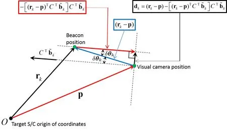
Figure 1:Problem geometry

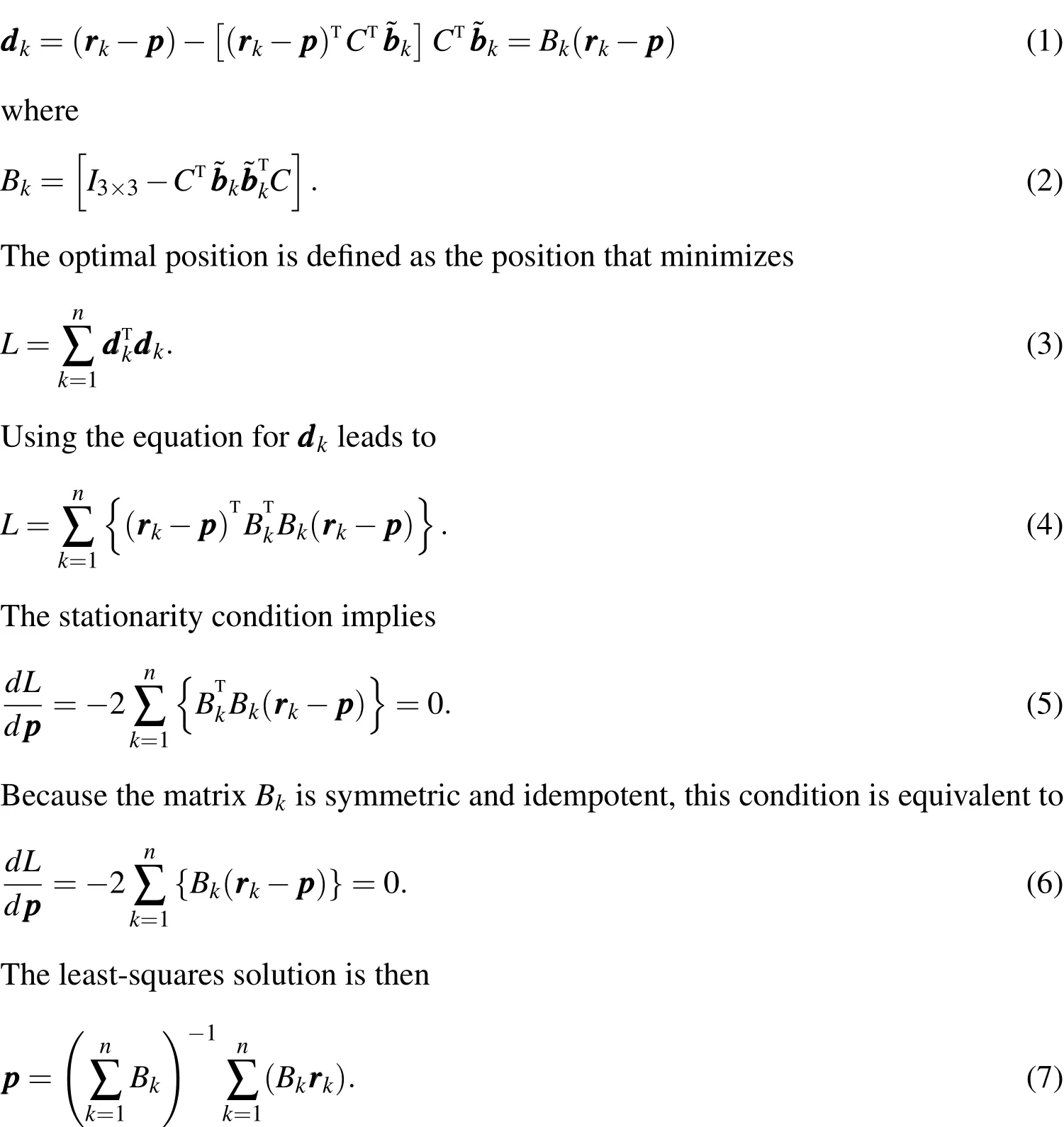
For the solution to be a minimum,the second derivative of the cost function with respect to the position must be positive definite.This is true when two or more non-collinear measurements are made.

3 Weighted least-squares single-point position estimation

The previous least-squares solution was optimal in the sense of an arbitrary cost function.This solution can be modified to obtain a statistically optimal estimate in the maximum likelihood sense.The steps for this derivation are as follows.First an error model for the measurements is given.Next,it is shown thatis a zero-mean Gaussian vector with specified covariance when conditioned on the true positionppp.Finally a solution for the position that maximizes the joint likelihood of all theis shown.

An approximate model for the measurement error is

This enables a convenient Maximum Likelihood Estimate(MLE)to be derived.The MLE minimizes the following cost function which is proportional to the nega-tive log-likelihood(neglecting constants).

where(A)+represents the pseudo-inverse of any matrixA.As is pointed out in Cheng,Crassidis,and Markley(2006),a rank-one update can be applied to the singular-covariance matrix to make it invertible with a near-zero impact on the cost function.The intuitive rational for this update is as follows.Because the covariance matrix foris rank-two,it implies that the component of the vectorin the direction of the null space of the covariance is zero.This null spaceis directed along the vectorTherefore,addingCfor any scalarto the covariance in the cost function will not change the cost since there is no component ofalong this direction anyway.To make the inverse of the updated covariance most sTtable,the eigenvalue of the updated covariance associated with the eigenvectorcan easily be set to the average of the other two eigenvalues which means that

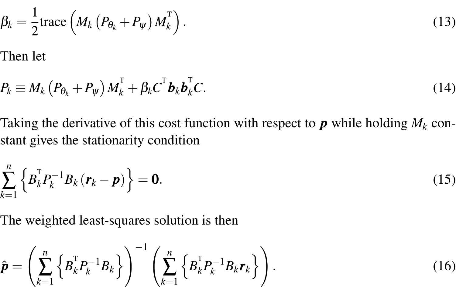
This is inherently an iterative solution.We must first use the unweighted least squares estimate to get an initial estimatewhich can then be used to get an initial estimate of theMkmatrices.This in turn is used to estimate a newand the process is repeated.Numerical tests demonstrate that at most two iterations of the weighted least squares are needed in all test cases.

A clear connection between this solution and the unweighted least squares solution can be seen as follows.Consider the case whenThen the covariance of(which is positive semidefinite).Looking at the equation fordddksuggests that it should be nearly orthogonal towhen the measurement errors are small.Then,for the purposes of the cost function,the covariance can be effectively replaced bywhich is similar to the results in Shuster(1990).The new cost function is then

which leads to the iterative solution

Because the true position is unknown,the weights must be determined iteratively.The unweighted solution is used to obtain an initial guess for position which is used to compute the initial weights. The is repeated iteratively, updating the weights with each new position estimate so that the weights on iterationℓused to compute the estimateare

In the numerical tests below,the measurement and attitude errors are assumed to be isotropic.Therefore we use Eq.(18)to generate the estimates.However,Eq.(16)could be used in the case of non-isotropic errors.

3.1 Error Covariance

Once the position estimate converges(typically after 1-2 iterations),a first order approximation to the error covariance can be computed.The first step in deriving the covariance equation is to decompose theBkmatrix defined in Eq.(7)into two components:one with and one without error.

Substituting Eq.(20)into Eq.(18)and approximating to first order gives the position estimate in terms of the truematrix and its errorδB.

Taking the expected value of this equation shows that the estimate is unbiased if the measurement errors are all zero-mean.In addition,the error covariance matrix can be found using Eq.(24).

The equation can be evaluated using the measuredBkinstead of the(unknown)trueThis equation is verified in the next section.

4 Numerical Examples

The companion paper to this one,Mortari and Conway(2015),demonstrates several properties of the weighted least squares algorithm.It is shown that one iteration of weighted least squares can reduce the position estimate error by a factor of 2 to 3 compared to the unweighted algorithm.In addition,it is shown that the weighted least squares method converges in only 1 to 2 iterations.Lastly,it is shown that the weighted version is much more robust to large variations in the sensor-to-target distances.

This paper presents analysis demonstrating clear advantages of the proposed algorithm over existing methods.The following numerical tests answer the following important questions about the proposed algorithm’s performance:

1.Is the proposed algorithm better than the typical image-space MLE approach?

2.Is the covariance expression statistically consistent with numerical results?

3.In the context of space-vehicle navigation,is it better to compute a coupled position and attitude estimate when star measurements are available or to decouple the solution(proposed algorithm for position and image-space MLE for attitude)?

4.1 Comparison to Image-Space Error Minimization

The traditional approach to position estimation from image measurements is to perform a minimization of the image-space reprojection errors.If the pixel measurements contain additive zero-mean Gaussian noise,then this algorithm gives the MLE[Hartley and Zisserman(2003)].This will be referred to as the image-space approach since it is the MLE when the assumed noise model is defined in imagespace as opposed to the proposed method which is the MLE when the assumed noise model is in object-space.The following example will compare the imagespace approach to the proposed approach over a test matrix of measurement error variances and number of landmarks.To obtain a fair comparison,the example is repeated twice:once for a simulation with the small rotation error model(used to derive the proposed method)and once for a simulation with the image-space additive noise model(used to derive the image-space method).

For each entry in the test matrix(i.e.for some image-space error covariance and landmark count),Ntrialsare performed.For each trial,the landmarks are generated uniformly random over a plane(sized to fit a 40◦FOV)in front of the camera and normal to the camera optical axis.The image-space and proposed method are applied to simulated measurements and the norm of the error for each algorithm is recorded.

Using the resulting Ntrialserror norms for both algorithms at a particular grid point,a Wilcoxon Signed-Rank Test(WSRT)is performed to test the null hypothesis that the mean error norm is the same for both methods[Boslaugh(2012)].The WSRT is a nonparametric hypothesis test for paired samples[Wilcoxon(1945);Siegel(1956)].A nonparametric method is needed for this test because the distribution of error norms is highly non-Gaussian.In addition,a paired samples test is desired to obtain a higher statistical power(lower risk of a false-negative).The data is paired in the sense that both position estimation algorithms are applied to the same simulated measurement(and underlying measurement error sample).The WSRT satisfies both of these criteria.

As with any hypothesis testing,it is critical to select Ntrialslarge enough to obtain sufficient statistical power.A simple Monte Carlo simulation is performed to find a suitable choice ofNtrials.In this test,two sets ofNtrialszero-mean Gaussian 3×1 vectors are generated with covarianceIt is found that the WSRT rejects the null hypothesis 99.9%of the time at a 0.05 significance level whenIn other words,if there is a difference in error distributions that is large enough to be of concern(more than 5%),then it is very likely(99.9%)that the hypothesis will be rejected for the chosen significance level(0.05).

The WSRT statistic for largeNtrialsis well-approximated by a Gaussian distribution.The variance of this distribution is a simple function ofNtrials.Therefore the Cumulative Probability Distribution(CDF)value for the test statistic can be obtained.Tab.1 displays the CDF value,mean error norm difference,and the sample standard deviation of the error norm difference.Using a significance value of 0.05,if the CDF value is less than 0.025 then we reject the null hypothesis for the alternative hypothesis that the proposed algorithm is better than image-space method(i.e.lower error norms).If on the other hand,the CDF value is greater than 0.975 then we reject the null hypothesis for the alternative hypothesis that the image-space method is better than the proposed algorithm.Note that this significance level is arbitrary but commonly used[Craparo(2007)].Tab.1 suggests one clear trend:the proposed method outperforms the image-space method for accurate sensors(σ＜0.3◦)while the image-space method outperforms the proposed method for less accurate sensors(σ≥0.5◦).This is true for both error models.This trend is likely a natural result of the different cost functions used to derive the methods.The proposed method minimizes the weighted sum of squares of objectspace errors which is directly related to our true objective:the best object-space position estimate.However,because the object-space errors are not additive Gaussian(higher order terms were dropped),the proposed method is not an exact MLE.This effect becomes more pronounced for larger measurement errors because the neglection of higher order terms in Eq.(9)becomes less and less appropriate.On the other hand,for smaller measurement errors,the linearization does hold and the direct relationship between the object-space errors and position estimate error makes the proposed method more attractive.

4.2 Covariance Consistency

The covariance expression in Eq.(27)is validated through a statistical analysis as follows.One Monte Carlo test withNtrials=10,000 trials is performed for the case of no attitude error(Pψ=0).For each trial,the number of observed point-targets is uniformly random betweenn=5 andn=10.The measurement error standard deviation is set toσ=0.1◦for all measurements.The point-target locations are generated uniformly random in the 3D unit-cube centered at a point three distanceunits in front of the sensor(along the positive z-axis).The simulated measurements are used to estimate the position and corresponding error covariance:The resulting erroris then transformed toare the eigenvalue and eigenvector matrices ofrespectively.The transformed errorshould be a zero-mean normal random variable with identity covariance ifPis the correct covariance forTo test this hypothesis,an unbiased estimate of the covarianceis computed.The variance of the components ofSare computed and used to compute a p-value for each component

ofS[Seber(2009)].Note that the p-value is the value of the inverse-CDF of the test statistic under the assumption that the null-hypothesis is true.The results are given in Tab.2.

Table 1:Test results for the hypothesis that the image-space and object-space approaches have the same mean position error norm.The test statistic CDF value,the mean error norm difference(proposed method minus image-space method),and the standard deviation of error norm differences,for various noise variances and target-landmark numbers,Nt.A near-zero(near-unity)CDF value indicates either an outlier test statistic was found or that the proposed method has a lower(higher)error norm mean than the image-space method.

Table 3:Expected and resulting covariance results with their corresponding errors,variances,and p-values.A random attitude error is given to the camera on each trial.Note a p-value≤0.025 or≥0.975 would suggest an inconsistency in the covariance for a two-sided test.

Tab.2 shows that the p-value for all six of the unique elements ofSis greater than 0.025 which does not provide strong evidence to reject the hypothesis.Furthermore,because the large number of trials produced a low standard deviation of 0.0137,we can conclude that the power of this statistical test is high enough to resolve a discrepancy inSthat may be of practical concern.

The same test used to generate the results of Tab.2 is repeated with the one difference being a simulated random attitude error with standard deviationσ=0.025◦about each axis.This attitude error is independently generated for each trial of the test.The results of the test using Eq.(27)are given in Tab.3.The main conclusions drawn from the numerical analysis in Tab.2 are analogous to those of this analysis:the covariance equation is numerically consistent with the numerical results The added value of the analysis results of Tab.3 is verification that the attitude error covariance can be directly accounted for in computing the resulting position error covariance.

4.3 Coupled vs.Decoupled Estimation

In theory,simultaneously estimating both position and attitude can give a better result than estimating them independently(because the image measurements of landmarks depend on both position and attitude).An MLE can be derived that uses image measurements of both stars and landmarks(point-targets at infinity and not at infinity).However,decoupling the solution has its advantages.The first advantage is a lower computational cost.The second advantage is that it is easier to apply robust estimation techniques to two small problems(decoupled estimation)as compared to one large problem(coupled estimation).Robust techniques are important in removing potential correspondence errors which may occur in visual navigation tasks.If the accuracy gains associated with the coupled solution are relatively small,then the advantages listed above may justify decoupling the solution.The following numerical example will demonstrate what type of accuracy gains can be achieved with this result.

A Monte Carlo analysis of 10,000 trials is performed.For each trial,it is assumed that a 30◦FOV star camera measures 5 stars with σstar=0.05◦error and a second 40◦FOV camera(oriented 90◦from the first)measures 5 landmarks with σbeacon=0.5◦error.These error values are typical of practical sensors.Note that an image of a star can be centroided with much greater accuracy than a landmark because of the much larger contrast between a star and its black background compared to the contrast between a beacon and the spacecraft it is mounted on for example.In each trial,the landmarks are uniformly randomly generated on a planar region located one distance unit in front of the camera and normal to the camera axis.The planar region is sized to fill up the camera FOV.Similarly,the stars are uniformly randomly generated over the star camera FOV.

The coupled solution is a MLE for position and attitude solved iteratively with a Levenberg-Marquardt method.Both stars and landmarks are used in this estimator.The decoupled solution first uses a Levenberg-Marquardt method to get a MLE for attitude.Only the star measurements are used in estimating attitude.The decoupled solution then uses this attitude estimate in the proposed method to compute the position.The results of this are shown in the histogram of Fig.2.

Figure 2:Error histogram for position(as a percent of the camera-to-landmark plane distance)and attitude estimates in the coupled(blue)and decoupled(red)solutions.

The results of Fig.2 show thatthere are no significant gains to be made from using a coupled solutionfor the specified sensor parameters in this test case.The primary reason for this is that star measurements can be made much more accurately than landmark measurements.Therefore the landmark measurements provide almost no new information about the attitude when conditioned on the star measurements.This effect is further exaggerated by the fact that position errors are coupled into any attitude information that a landmark measurement can provide.

5 Relative Position Filter

This section will demonstrate the use of the weighted least-squares algorithm in a sequential filtering framework to fuse inertial and visual measurements.The traditional approach to filtering with visual measurements of surveyed points is to use an Extended Kalman Filter(EKF).The EKF measurement update can treat each landmark individually,similar to the attitude filter of Crassidis and Junkins(2012).The alternative presented here is to use the proposed algorithm as a preprocessing step on the individual landmark measurements.The position estimate from the algorithm,along with the associated covariance,can then be treated as the measurement input to the filter.The advantage of this approach is that the measurement input to the filter is linear in the filter states.This overcomes the well known disadvantages of the EKF,namely corrections that are only accurate to first order and inconsistency of the covariance estimate with the actual error statistics.

In the following,some notation is first introduced.Then the filter equations are derived.Lastly,a numerical example is shown.

5.1 Notation and Reference Frames

The vector from the origin of frameato the origin of framebwith components along framecis denoted by(i.e.“b relative to a in c”).The rotation matrixCb/atransforms the coordinates of a vector in frameato frameb:

A single subscript is used to indicate the time dependence.For example,Piis the state covariancePat timeti.

The estimate and measurement of a true quantityxare represented byˆxand˜xrespectively.For rotation matrices,the true rotation matrix is represented in terms of its estimate and some small error as

The following reference frames will be used:

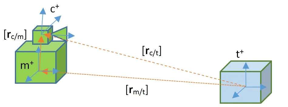
Figure 3:Reference frames

The rigid transformation between themandcframes is assumed to be known from a prior calibration.The target vehicle is assumed to have its own Inertial Navigation System(INS)that can send estimates of thetframe attitude relative to thenframe.The target vehicle can also send it’s own IMU data to the docking vehicle.

The filter state consists of the relative position and velocity between the docking and target vehicle,and the docking vehicle accelerometer bias.In particular:

5.2 Kinematics

The state vector evolves according to the following differential equation

The accelerometer bias is a random walk process with covarianceThe acceleration termcan be computed using the accelerometer outputs.The docking vehicle accelerometer outputis the sum of the inertial acceleration of the IMU center, a bias term, and a zero-mean noise term with components in the IMU frame.

In order to propagate the state,the accelerometer outputs must be related to using the current estimate of bias and local gravity as

The estimate is then propagated by integrating

5.3 Error Kinematics

The error state is the difference between the estimated and true state:The covariance of the state error isIn order to propagate the state error covariance matrix,the difference between the true and expected rates given in Eq.(29)and Eq.(32)must be linearized in terms of the current state errorsand other sources of noise.The resulting continuous time error kinematics in matrix form are

5.4 Measurement Update

Images are processed to extract the pixel locations of surveyed landmarks on the target vehicle.The camera calibration matrix,K,and the IMU-to-camera rotation,are used to convert the pixel locations into unit vectors in the m frame.Letbe the i-th surveyed landmark in the target vehicle frame.The corresponding measured 2D pixel location isThe measured unit vector is

Note thatγis used to normalize the vector to unit length.Given some error covariance on the pixel measurement,Rui,the error covariance on the unit vector is

A set ofNmeasurements,namely the known landmark position,measured unit vector,and error covarianceis passed to the weighted least squares algorithm.The output isand a corresponding error covariance(defined asrespectively in the previous sections).To incorporate this into the filter,the measurement is expressed in terms of the filter states as

5.5 State Update

A state update is performed each time a new measurement and its covariance are computed using the standard Kalman Filter equations[Crassidis and Junkins(2012)].First the Kalman gain is computed.

Then the state update is computed using the difference between the measured and expected target-to-camera position.

This update is applied to the current state estimate and the posterior state covariance is computed.

Note that the symmetry in the covariance can be explicitly enforced if necessary.

5.6 Numerical Example

To demonstrate the use of the position estimator,the filter is applied to the problem of space vehicle docking.Other authors have investigated and applied visual measurements to the docking problem both in air[Valasek,Gunnam,Kimmett,Junkins,Hughes,and Tandale(2005)]and in space[Ho and McClamroch(1993);Kim and Rock(2009)].Specific systems have been proposed for visual point-targets that can be reliably detected in a space environment[Bondy,Krishnasamy,Crymble,and Jasiobedzki(2007)].In the example below,two vehicles are in 8,000 km near-circular orbits about Earth.The target vehicle(TV)initially leads the docking vehicle(DV)by≈100mand reduces this distance to≈15mover 50s.The DV propagates its state at 10 Hz using its own IMU data and the accelerometer data from the TV.

The state update uses camera measurements at 2 Hz that are simulated for a 1024×1024 pixel sensor with a 26◦×26◦field-of-view.The TV has 20 beacons,some of which may not be visible at all times.The 1σpixel noise is set to 9 pixels which corresponds to 1◦error.

The resulting trajectory of the true and estimated states is shown in Fig.4.To see more detail,the filtered estimate errors over the first 10 seconds are shown on the top of Fig.5 and from a ten second segment in the middle of the run(which is representative of the steady-state performance)is shown on the bottom of Fig.5.Note that the initial errors are on the order of 10mand 1m/sfor position and velocity respectively.The errors converge to around 0.05mand 0.05m/srespectively.The solid lines represent the actual errors while the dashed lines represent the computed error bounds.Note that the diamonds indicate the actual position measurement errors.

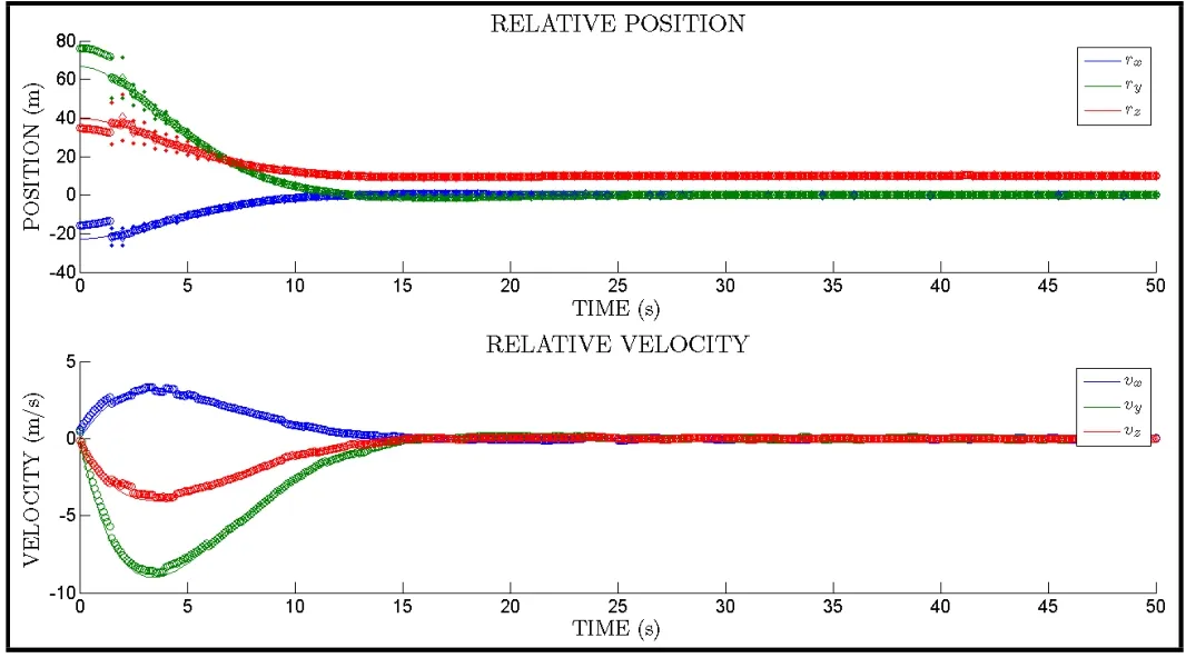
Figure 4:True(solid line)and estimated(dashed line)position and velocity.The measured position is shown in the top plot(diamonds).

Figure 5:Position and velocity errors and 3σ bounds in first 10 seconds(left)and a 10 second segment in the middle of the test(right).

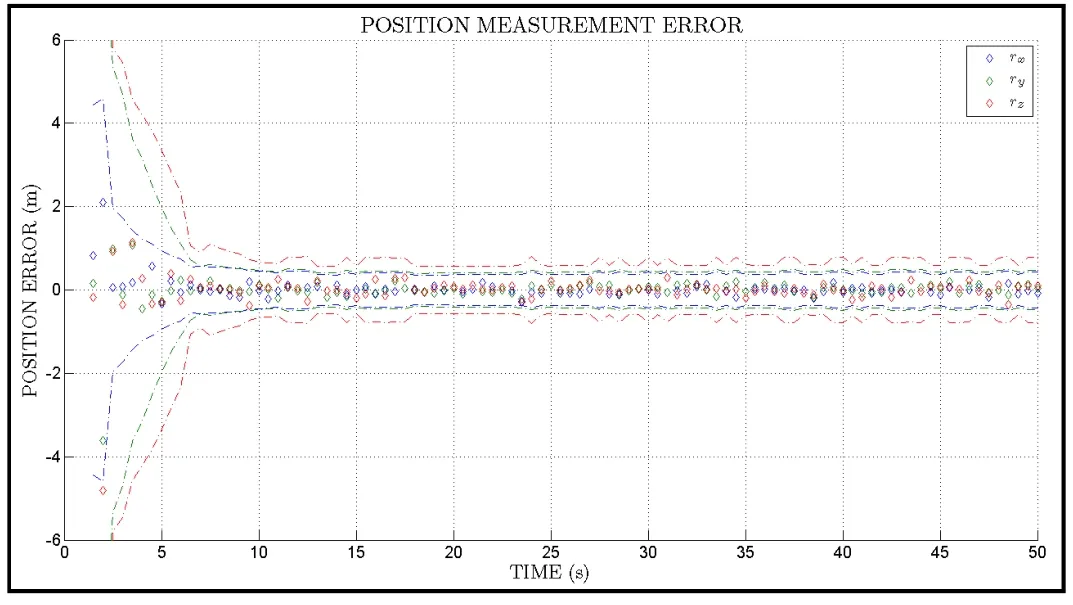
Figure 6:Measurement error and 3σ bounds(single-point estimates).

Fig.6 shows the position measurement(i.e.single-point position estimate indepen-dent of filter)errors in more detail.The dashed lines in Fig.6 show the computed error bounds and the diamonds show the actual errors.Two important facts should be noted.First,the errors in the beginning of the run are larger primarily due to the fact that the camera-to-target distance is larger in the beginning of the run(i.e.the position estimates become more accurate as the vehicles get closer:a very desirable property).Second,the computed bounds agree very well with the errors.This is consistent with the results in Tab.2.

6 Conclusions

This paper presents a novel solution to the problem of determining position from 2D-to-3D correspondences when the attitude is known.The case of known attitude is common in applications like navigation where other sensors can provide accurate attitude estimates.Compared to previously published solutions(when modified for the case of known attitude),the proposed method has several unique advantages.First,it can easily take into account different image-space error variances and camera-landmark distances.Second,because the cost function is defined in terms of object-space error,the resulting position estimate can be better than those of a image-space MLE as shown in the Numerical Analysis section.Third,the proposed position estimator can give nearly the same accuracy as a coupled attitude and position MLE for practical sensors but at a much lower computational cost.The proposed method has a lower cost-per-iteration than a coupled MLE and requires only two iterations while the coupled MLE requires 8-10 iterations.The computational complexity isO(n)fornpoints and only a 3×3 linear system must be solved.This also makes the algorithm very easy to implement.

The proposed method has an accurate covariance expression for the estimate error(in terms of measurement and attitude error)which enables sequential filtering applications.The estimator can easily be incorporated into a filtering framework as has been demonstrated.In a filter,the proposed solution can be treated as a direct measurement of the position with known error covariance.This significantly reduces filter complexity compared to the case of using the individual pixel locations as measurements.It can also improve robustness when used in conjunction with robust estimation techniques like RANSAC.For example,two measured pointtargets can be randomly selected from the set of all measurements at a given time.The proposed algorithm can be used to quickly compute a position estimate under the hypothesis that the selected measurements are valid(i.e.not gross outliers).The estimated position can then be used to check the residual of all other measurements to find an inlier set.This process can be repeated many times to find the largest inlier set(i.e.the largest consensus).The largest inlier set can then be used to compute the final position estimate.The speed and accuracy of the proposed algorithm is especially useful in this context.The weighting scheme proposed in this work can also be applied to other problems in photogrammetry to improve robustness and accuracy in a statistical sense.This will be a focus of future work.

Acknowledgement:The authors would like to thank the NASA Space Technology Research Fellowship program for supporting this work.The authors would also like to thank the reviewers for their effort and valuable comments.

Bondy,M.;Krishnasamy,R.;Crymble,D.;Jasiobedzki,P.(2007): Space vision marker system(svms).InAIAA SPACE 2007 Conference and Exposition,pp.18–20.

Boslaugh,S.(2012):Statistics in a nutshell."O’Reilly Media,Inc.".

Cheng,Y.;Crassidis,J.L.;Markley,F.L.(2006):Attitude estimation for largefield-of-view sensors.The Journal of the Astronautical Sciences,vol.54,no.3-4,pp.433–448.

Craparo,R.M.(2007):Encyclopedia of measurement and statistics:Significance level,2007.

Crassidis,J.L.;Junkins,J.L.(2012):Optimal Estimation of Dynamic Systems.CRC Press.

Gao,X.-S.;Hou,X.-R.;Tang,J.;Cheng,H.-F.(2003):Complete Solution Classification for the Perspective-Three-Point Problem.Pattern Analysis and Machine Intelligence,IEEE Transactions on,vol.25,no.8,pp.930–943.

Hartley,R.;Zisserman,A.(2003):Multiple View Geometry in Computer Vision.Cambridge University Press.

Ho,C.-C.J.;McClamroch,N.H.(1993):Automatic Spacecraft Docking Using Computer Vision-Based Guidance and Control Techniques.Journal of Guidance,Control,and Dynamics,vol.16,no.2,pp.281–288.

Horn,B.K.(1987): Closed-form solution of absolute orientation using unit quaternions.JOSA A,vol.4,no.4,pp.629–642.

Kim,J.;Rock,S.(2009):Feedback dual controller design and its application to monocular vision-based docking.Journal of guidance,control,and dynamics,vol.32,no.4,pp.1134–1142.

Lepetit,V.;Moreno-Noguer,F.;Fua,P.(2009): EPNP:An AccurateO(n)Solution to the PNP Problem.International journal of computer vision,vol.81,no.2,pp.155–166.

Lu,C.-P.;Hager,G.D.;Mjolsness,E.(2000): Fast and Globally Convergent Pose Estimation from Video Images.IEEE Transactions on Pattern Analysis and Machine Intelligence,vol.22,no.6,pp.610–622.

McReynolds,D.P.(1988):Solving for Relative Orientation and Depth.PhD thesis,University of British Columbia,1988.

Mortari,D.;Conway,D.(2015):Single-point Position Estimation in Interplanetary Trajectories Using Star Trackers.InAIAA/AAS Astrodynamics Specialists Conference,Vail,CO.

Seber,G.A.(2009):Multivariate observations,volume 252.John Wiley&Sons.

Shuster,M.(1990):Kalman filtering of spacecraft attitude and the quest model.Journal of the Astronautical Sciences,vol.38,pp.377–393.

Siegel,S.(1956):Nonparametric statistics for the behavioral sciences.

Valasek,J.;Gunnam,K.;Kimmett,J.;Junkins,J.L.;Hughes,D.;Tandale,M.D.(2005): Vision-based sensor and navigation system for autonomous air refueling.Journal of Guidance,Control,and Dynamics,vol.28,no.5,pp.979–989.

Weng,J.;Ahuja,N.;Huang,T.S.(1993):Optimal Motion and Structure Estimation.IEEE Transactions on Pattern Analysis and Machine Intelligence,vol.15,no.9,pp.864–884.

Wilcoxon,F.(1945): Individual comparisons by ranking methods.Biometrics bulletin,pp.80–83.

1PhD Student,Aerospace Engineering,Texas A&M University,College Station,77843.E-mail:dtconway@tamu.edu.

2Professor,Aerospace Engineering,Texas A&M University,College Station,77843.

E-mail:mortari@tamu.edu.