Transition study of 3D aerodynamic configures using improved transport equations modeling

Xu Jiakuan,Bai Junqiang,Zhang Yang,Qiao Lei

School of Aeronautics,Northwestern Polytechnical University,Xi’an 710072,China

Transition study of 3D aerodynamic configures using improved transport equations modeling

Xu Jiakuan,Bai Junqiang*,Zhang Yang,Qiao Lei

School of Aeronautics,Northwestern Polytechnical University,Xi’an 710072,China

As boundary layer transition plays an important role in aerodynamic drag prediction,the proposal and study of transition prediction methods simulating the complex flow phenomena are prerequisite for aerodynamic design.In this paper,with the application of the linear stability theory based on amplification factor transport transition equations on the two-equation shear stress transport(SST)eddy-viscosity model,a new method,the SST-NTS-NCFmodel,is yielded.The new amplification factor transport equation for the crossflow instability induced transition is proposed to add to the NTSequation proposed by Coder,which simulates Tollmien–Schlichting wave transition.The turbulent kinetic energy equation is modified by introducing a new source term that simulates the transition process without the intermittency factor equation.Finally,coupled with these two amplification factor transport equations and SST turbulence model,a four-equation transition turbulence model is built.Comparisons between predictions using the new model and wind-tunnel experiments of NACA64(2)A015,NLF(2)-0415 and ONERA-D infinite swept wing and ONERAM6 swept wing validate the predictive quality of the new SST-NTS-NCFmodel.

1.Introduction

With the development of experiment technology,the details of boundary layer transition flows had been researched and revealed very well.1,2In the meantime,the compatible way for engineer application-computational fluid dynamics(CFD)method,is gradually applied and developed for the drag prediction of boundary transition for the aerodynamic design of aircraft.Prediction of boundary layer transition is an important part in the simulation of boundary layer flows because lift and drag are significantly influenced by the transition locations.In 2D boundary layers,bypass transition,laminar separation bubbles and Tollmien–Schlichting(TS)wave always lead to transition.But in 3D boundary layers,crossflow instability usually play an important role in triggering the transition,especially for the swept wing with large swept angle.The prediction of transition phenomenon has an important meaning for aerodynamic calculations.There fore,it is necessary to study and establish a new method to simulate these transition phenomena.To predict these phenomena numerically,an appropriate approach would probably be large eddy simulation(LES)or direct numerical simulations(DNS).But these methods cost huge computational resources.So it could not be used in engineering application.

In recent years,many methods were proposed to predict boundary layer transition based on Reynoldsaverage Navier–Stokes(RANS)method.A model for bypass and natural transition prediction using the laminar kinetic energy transport equation was proposed by Walters et al.3–5In 2004, Langtry and Menter developed thecorrelation-based transition model6–8using local variables which are coupled with Menter’s two-equation k-ω shear stress transport(SST)turbulent model.9This transition model,which could predict the natural transition,laminar separation transition and the bypass transition,is widely applied in engineering field.10,11But these methods could not predict the cross flow instability induced transition.

In aviation field,a widely used method in applied aerodynamics is the eNmethod which is based on linear stability analysis,specifically the eNmethod proposed by Smith and Gamberoni12and Van Ingen13.The eNmethod14is basically designed for 2D boundary layers and can be extended to 3D boundary layers,but it still exhibits some deficiencies.A major disadvantage of this method is that the N-factor,which is responsible for a critical amplification of linear disturbances,has to be fit to each test case.Additionally,the application of the eNmethod for a RANS code is complicated due to thefact that some non-local variables need to be solved.Integral boundary layer quantities are gradually solved by some other local variables.

In 2013,the streamwise amplification factor equation15for TS wave instability has been applied to the Spalart–Allmaras(SA)one-equation eddy-viscosity model16.The equation was validated by using many con figurations in Ref.15But this model is still under development and not impeccable for the cross flow instability induced transition on swept wings.In this paper,the Falkner-Skan-Cooke(FSC)17boundary layer similar equations and linear stability theory(LST)were used to analyze the crosswise velocity pro files and to establish a new amplification factor transport equation for prediction of cross flow instability.Fig.1 shows a series of cross flow velocity profiles of 45°swept wing in various pressure gradients calculated by FSC equations.In Fig.1,η is the non-dimensional distance normal to the wall,w the non-dimensional cross flow velocity and βHrepresents the Hartree pressure gradient.

Fig.1 Crossflow velocity profiles on swept wings.

For the transition equations coupling with turbulence model,the qualities of the SA model,in particular its turbulence-suppression function used in conjunction with user-specified trip lines,allow transition to be included without the addition of an intermittency transport equation.15This stands in contrast with the widely implemented transition framework of Langtry and Menter6–8,which uses such a transport equation.

Finally,it is desirable to apply the two amplification factor transport transition equations(including NTSand NCFequations)to the SST turbulence model.A turbulent kinetic energy production term18was chosen without using an intermittency transport equation so that the two amplification factor transport equations are coupled with SST turbulence model for transition prediction of 3D aerodynamic configuration.

2.Amplification factor transport equation modeling

2.1.New NCFamplification factor transport equation governing equation

With the study of Coder’s model15,the approximate envelope mNethods of Gleyzes et al.19and Drela and Giles20simplify the emethod by tracking only the maximum amplitude of the most-amplified frequencies and assuming linear amplitude growth with locally self-similar boundary-layer development.15Using the approximate envelope method for analysis of crossflow stationary vortices,the envelop amplification factor NCFof the cross flow instabilities is determined as

The integrand characterizes the spatial growth rate of the instability and depends entirely on the local boundary-layer shapefactor and crosswise displacement thickness ReδCF.Similar to NTSequation,the crosswise amplification factor transport equation is proposed:

The source term Pn，CFof this equation is a function of streamwise shapefactor H12calculated by a local pressure gradient parameter HLthrough the Falkner-Skan profiles.The coefficient of diffusion term σn，CFis equal to 1.0.In Eq.(2),μ and μtare laminar viscosity value and eddy viscosity value respectively.The source term Pn，CFis

where Ω is the absolute value of vorticity,ρ the density,fkthe control function,fk=exp［-（RT/2.0）20］,RTthe viscous ratio,RT= μt/μ.Thefunction Ngrowth,CFof source term Pn，CFis a combination of correlations to describe the shape-factor dependency of the local boundary-layer growth rate in the crosswise direction.This function is defined as in Eq.(4)and obtained by the FSC velocity profiles.It relates the inflection of local crossflow velocity along the streamwise pressure gradient HLand streamwise shapefactor H12.

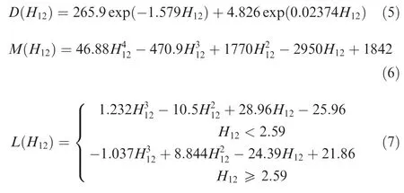
where the three parts of function Ngrowth,CFwere similar to that of Coder’s model,but they werefitted afresh for crossflow velocity profiles.M（H12）and L（H12）werefitted to describe the growth of the crosswise displacement thickness in Falkner-Skan-Cooke boundary layers.The D（H12）correlation has been developed as the damping function and relates the crosswise displacement thickness using the FSC similarity velocity profiles.They are all functions of streamwise shapefactor H12and expressed as

The Fcrit，CFfunction of source term Pn，CFis used to determine the unstable position of crossflow instability mode in boundary layer and defined as

Fig.2 Solution of local crossflow velocity.

where the constant Cz=10.0,Rez=.For swept wing,the cross flow velocity UCFiscalculated using the formula UCF=UsinΔ and the angle could be given by Δ =Λc-Λ+ΛGwhere ΛGis the geometry sweep angle,Λ=arctanthe local sweep angle,and Λcis given by arctan（v/u）.In preceding formulas,Cpis pressure coefficient,u and v are Cartesian velocity components in the x-and zdirections respectively.These variables are illustrated in Fig.2 which contains the velocity normal to the leading edge Uc,the velocity component in the span-wise direction Ws,the velocity at boundary layer edge Ue,the stream-wise component velocity U and the crosswise component velocity W(corresponding to UCF).Using this method,the crossflow velocity UCFcould be calculated locally.If the configuration is complex,the redefined coordinate system method proposed by Choi and Kwon21could be used here to calculate the new swept angle under assumption that there is no pressure gradient in the spanwise direction.22Furthermore,the local flow velocity is used to define the reference coordinate system instead of the external potential flow direction,which could be adopted to estimate crossflow velocity UCFapproximately.ReδCF，0is the critical crosswise displacement thickness Reynolds number.is the development slope of NCFcalculated through the FSC velocity pro files and linear stability theory in infinite swept status which is in spatial pattern.Because the traveling crossflow mode is prone to dominant appearance in the presence of larger freestream disturbances,the stationary crossflow vortices is the major mode of swept wing in high fight altitude or low turbulence intensity tunnel.So the stationary mode is the key point of our research.For infinite swept wing,the time amplification rate ωiis 0 and the spanwise disturbance amplification rate βiis 0 according to the Mack’s method.23Also both thefrequency f and ωrare 0 for the analysis of crossflow stationary vortices.So the calculation is simplified to a great extent.β is the spanwise disturbance wavenumber.A series of β was used to calculate the critical crosswise displacement thickness Reynolds number and the slope of most unstable disturbance wave for each shapefactor H12.Thefunction Cm（H12）is obtained by the FSC velocity profiles.

2.2.Application to k-ω SST turbulence model

From Refs.24,25,DNS data demonstrates that all small vortices are generated by multilevel shear layers,not by vortex breakdown in the transition region.This is a new theory to explain and analyze the development of boundary layer transition.So it inspired the authors that the intermittency factor is not necessary to be used to govern the transitional flow.The intermittency factor could be replaced by other suit methods.From Ref.18,we can use theft2function to be a suitable algebraic substitute to the transported intermittency factor.The new amplification factor equation was coupled with SST turbulence model by the new production term for turbulence kinetic energy k equation:

where

The constant ct5=0.5,ct4=0.05 and κ=0.41.S is the absolute value of strain rate,d the distance to the nearest wall and Χ the modified eddy viscosity ratio18:

The F1function is defined using the extended form proposed by Langtry and Menter8

The critical value NTS，crit=-8.43-2.4lnproposed by Mack23and it is recommended that NTS,critco

uld be limited to nine in general applications for both numerical reasons.Thefact that NTS,crit=9.0 works well for engineering purposes when there is very low freestream turbulence.For the crossflow amplification factor,the critical value of NCF,critvaries from 6.5 to 8.0 and usually 7.0 is chosen.

2.3.Final equations

The present model(named NTS+NCFmodel)consists of a transport equation for TS waves,a new transport equation for crossflow stationary vortices,and the equations for turbulence kinetic energy k and specific dissipation rate ω which are modified from the SST k-ω eddy-viscosity model and all of which are listed as follows:

The NTSmodel is composed of the transport equation for TS waves and the equations for turbulence kinetic energy k and specific dissipation rate ω.All of the variables in the turbulence kinetic energy k equation and specific dissipation rate ω equation can befound in the Ref.9.

3.Presentation of results

In the present work,an in-house structured Reynolds averaged Navier–Stokes solver is used as the baseline flow solver.The solver is capable of analyzing two-and 3D configurations in either time accurate or steady-state simulations using a variety of discretization schemes and time-marching algorithms.The spatial discretization involves a semi-discretefinite-volume approach.Upwind-biasing is used for the convective and pressure terms,while central differencing is used for the shear stress and heat transfer terms.Time advancement is implicit with the ability to solve steady or unsteady flows.Multi-grid and mesh sequencing are available for convergence acceleration with the message passing interface(MPI)parallelization computation.In this work,all of the transition prediction results are obtained by using the amplification factor transport equations coupling with the SST turbulence model.

3.1.NACA64(2)A015 infinite swept wing

The new amplification factor transport equation was applied to another infinite swept wing flow.The NACA64(2)A015 infinite swept wing test case was experimentally investigated by Boltz et al.in the Ames Research Center26.Thefreestream turbulence intensity of the wind tunnel is very low.Hence,9.0 is chosen for the NTS,critvalue.

The swept angle of 40°and the angle of attack α =-1°were chosen for validation.The transition locations were measured at Mach number Ma=0.27.Reynolds number Re varies from 4.8×106to 7.3×106in the wind tunnel.The number of grid elements in the wall-normal direction is 61;the chordwise resolution is 121 cells on either wing side.Here,y+(1)of the cell next to the wall is smaller than 1.0.

The grid sensitive study of NCFequation was per formed here to demonstrate the robustness of the new transition model.In this test,Reynolds number is 7.3×106.The baseline grid is the mesh whose maximum y+(1)is close to 1.0,referred to as the ‘fine”grid,with ‘medium”and ‘coarse” grids generated by successively controlling the maximum y+(1)close to 2.0 and 5.0 respectively.The development of skin friction coefficient Cfon upper surface for the three grids is plotted in Fig.3 that the horizontal ordinate x/c indicates the normalization location of section airfoil.The plotted curves show only a small difference in the transition location between the coarse and medium grids and show almost no difference between the medium and fine grids.The medium grid is there fore regarded as producing grid converged solutions.The lack of significant variation between the medium and fine grid solutions shows that true grid convergence is possible with this transition model and that continued refinement does not deteriorate the solution quality.

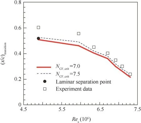
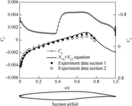
In this case,two critical values 7.0 and 7.5 were tested for these predictions,and it can be seen that NCF,crit=7.5 got better transition locations in Fig.4.For details,at the Reynolds number of 7.3×106,the pressure coefficient Cpand skin friction coefficient Cfof upper surface are plotted in Fig.5.Furthermore,Fig.6 shows the NCFand turbulence kinetic energy K contours around the NACA64(2)A015 infinite 40°swept wing at the Reynolds number of 7.3×106.It can be seen from the figure that,the transition occurred at near the 24%c position where NCFincreases to 7.5.

Fig.3 Predicted skin-friction distribution along streamwise section of upper surface of NACA64(2)A015 infinite swept wing.

3.2.NLF(2)-0415 infinite swept wing

The second case is the classical NLF(2)-0415 infinite swept wing which has been designed in order to investigate transition due to crossflow instability.These experiments were per formed in the wind tunnel at Arizona State University27.The freestream turbulence intensity of the wind tunnel was about 0.09%,so 8.4 is chosen for the NTS,critvalue.The NLF(2)-0415 airfoil was analyzed with the NTSequations proposed by Coder.The mesh is similar to that of NACA64(2)A015 wing.

The swept angle was 45°and the angle of attack is-4° for all related transition experiments.The transition locations were measured with naphthalene flow visualization technique,hot wire,and hot film measurements at Reynolds number varying from 1.9×106to 3.8×106in the wind tunnel.Once the Reynolds number was greater than 2.3×106,the transition process was assumed to be almost dominated by crossflow instability.If the equation for TS waves was used here,there would be a large difference of transition locations between the experimental data and CFD predictions.

The results of the computations of upper surface compared with the experiment data are plotted in Fig.7.The transition locations are shown depending on the Reynolds number.Computations were per formed with the Coder NTSequation and the present NTS+NCFequation.In Fig.7,it can be seen that the results of the present equations are in very good agreement with the experimental data.Nevertheless,compared to the Coder’s NTStransition prediction method which almost became invalid for these status,the results of NTS+NCFequations are very promising.Fig.8 shows the pressure coefficient and skin friction coefficient on the upper surface of NLF(2)-0415 infinite swept wing at the Reynolds number of 3.27×106and Mach number of 0.209.Fig.9 illustrates the pressure coefficient,skin friction coefficient and the streamlines on the upper surface of NLF(2)-0415 infinite swept wing at the Reynolds number of 3.72×106and Mach number of 0.238,which validate the accuracy of simulation of crossflow instability induced transition on swept wing compared to the experiment data.

Fig.4 Transition locations on upper surface of NACA64(2)A015 infinite 40°swept wing.

Fig.5 Pressure and skin friction coefficients of upper surface of NACA64(2)A015 infinite 40°swept wing at the Re=7.3×106,Ma=0.27,α=-1°.

3.3.ONERA-M6 swept wing and ONERA-D infinite swept wing

Finally,the new amplification factor transport equation was tested to the ONERA-M6 wing and the ONERA-D infinite swept wing which was experimentally investigated in the ONERA S2Ch low-speed wind tunnel.28,29

Fig.6 NCFand kinetic energy contours of upper surface of NACA64(2)A015 infinite 40°swept wing at Reynolds number of 7.3×106.

Fig.7 Transition locations on upper surface of NLF(2)-0415 infinite swept wing.

Fig.8 Pressure and skin friction coefficients of upper surface of NLF(2)-0415 infinite swept wing at Re=3.27×106.

Fig.9 Pressure and skin friction coefficients of upper surface of NLF(2)-0415 infinite swept wing at Re=3.72×106.

Fig.10 Laminar and turbulent regions on upper and lower surfaces of ONERA-M6 swept wing.

ONERA-M6 wing is a single element semi-span swept,tapered wing with an aspect ratio of 3.8 and a taper ratio of 0.562.The leading edge sweep angle is 30°and the trailing edge sweep angle is 15.8°.At the 25%line of the wing,this results in a sweep angle of 26.7°.The design of the wing was based on a symmetric airfoil using the ONERA-D section perpendicular to the 40%line.For ONERA-M6 wing experiment,the value of freestream turbulence intensity(FSTI)of the wind tunnel is about 0.2%.Measurements were per formed at Ma=0.262 and Re=3.5×106.The angle of attack varying from 0°to 15°were measured in the wind tunnel.

Fig.10 shows the depiction of the laminar and turbulent surface regions from the test showing the naphthalene distribution on the wing.For details,Fig.11 shows the transition locations of lower surface at the spanwise position zs/b=0.45 for different angles of attack on the lower side of the wing.For the numerical results,the transition locations were determined at the minimum of the skin friction coefficient distribution in the given spanwise wing section.The results show that the application of the SST+NTS+NCFmodel improves the accuracy of predicted transition location significantly.For an angle of attack of 5°,NCFcontour and kinetic energy contour of the spanwise section zs/b=0.45 are shown in Fig.12.It can be seen from thefigure that the transition occurred near the 32%c position of the lower surface where NCFincreases to 6.0.This transition location is very close to experiment data and prediction accuracy is significantly improved compared with Langtry’s transition model.

Fig.11 Transition locations for lower surface of ONERA-M6 swept wing at zs/b=0.45.

Fig.12 NCFand kinetic energy contours of spanwise section zs/b=0.45 of ONERA-M6 swept wing at α =5°.

Fig.13 Transition locations for upper surface of ONERA-D infinite swept wing.

For the ONERA-D infinite swept wing,the freestream turbulence intensity of the wind tunnel was about 0.2%.The angle of attack is α =-6°.The two Reynolds numbers,Re=1.0×106and Re=1.5×106were chosen to be measured in the wind tunnel.The swept angle varies from 0 to 60°and several swept wings due to crossflow instability were used to validated the present model here.In Fig.13,the transition locations for the ONERA-D wing for the NTS+NCFmodel are given in comparison to the experimental data.In addition,the NTSequation for TS waves was plotted,even though it is not designed for 3D transition phenomena.For all computations using different transition prediction methods,the Menter SST k-ω turbulence model was used.Compared to the experimental data,there are deviations of the computed results,but compared to the original NTSamplification factor equation,the results are very satisfying and promising.

Attention should be paid to the NCF,crithere.For ONERAM6 wing and ONERA-D infinite swept wing,NCF,crit=6.0 could get a better results and NCF,crit=7.0 would lead to a delayed transition position,so the value of NCF,critwas calibrated empirically.

4.Conclusions

The four-equation model has been established by two amplification factor transport equations for TS wave instability and crossflow instability transition incorporating linear stability theory based on the approximate envelope method and the SST turbulence model.The new model was confirmed by transition predictions of the infinite NACA64(2)A015 4°swept wing,NLF(2)-0415 infinite swept wing and ONERA-M6 wing.

(1)Solutions obtained for infinite swept wing and M6 wing using SST-NTS-NCFmodel agree well with experimental transition characteristics.The critical value of NCFmight influence the position of transition and it was calibrated empirically to get a better result.As is known to all,it can befound in many wind tunnel experiments that the critical values of NCFare case-sensitive.So it still needs to be researched further.

(2)Thesefavorable comparisons lend confidence in the transition equation,demonstrating that the intermittency factor equation could be supplanted by the new turbulent kinetic energy source term for interfacing between the transition and turbulence models.

(3)The development functions of crossflow instability are all obtained through the crossflow stationary vortices conditionally,so it still needs to be enhanced further for traveling waves.

In the future,the transition model as presented will be developed and applied to more complex aerodynamic configurations at high Reynolds number transition predictions and be extended for supersonic flows.

Acknowledgement

This study was supported by the National Basic Research Program of China(No.2014CB744804).

1.Lee CB,Wu JZ.Transition in wall-bounded flows.Appl Mech Rev 2008;61(3):030802.

2.Lee C,Li R.Dominant structure for turbulent production in a transitional boundary layer.J Turbul 2007;8(55):1–35.

3.Walters KD,Leylek JH.Computational fluid dynamics study of wake-induced transition on a compressor-like flat plate.J Turbomach 2005;127(1):52–63.

4.Walters KD,Cokljat D.A three-equation eddy-viscosity model for Reynolds-averaged Navier-Stokes simulations of transitional flow.J Fluid Eng T ASME 2008;130(12),121401-1-14.

5.Reza TZ,Mahmood S,Amir K.Prediction of boundary layer transition based on modeling of laminar fluctuations using RANS approach.Chinese J Aeronaut 2009;22(2):113–20.

6.Menter FR,Langtry RB,Likki SR,Suzen YB,Huang PG,Vo¨lker S.A correlation-based transition model using local variables Part I:model formulation.J Turbomach 2004;128(3):413–22.

7.Menter FR,Langtry RB,Likki SR,Suzen YB,Huang PG,Vo¨lker S.A correlation-based transition model using local variables Part II:test cases and industrial applications.J Turbomach 2004;128(3):423–34.

8.Langtry RB,Menter FR.Correlation-based transition modeling for unstructured parallelized computational fluid dynamics codes.AIAA J 2009;47(12):2894–906.

9.Menter FR.Two-equation eddy-viscosity turbulence models for engineering applications.AIAA J 1994;32(8):1598–605.

10.Wang YT,Zhang YL,Li S,Meng DH.Calibration of transition model and its validation in low-speed flows with high-order numerical method.Chinese J Aeronaut 2015;28(3):704–11.

11.Xia CC,Chen WF.Boundary-layer transition prediction using a simplified correlation-based model.Chinese J Aeronaut 2016;29(1):66–75.

12.Smith AMO,Gamberoni N.Transition,pressure gradient and stability theory.Long Beach(CA):Douglas Aircraft Company;1956,Report No.:ES-26388.

13.Van Ingen JL.A suggested semi-empirical method for the calculation of the boundary layer transition region.Delft:Delft University of Technology;1956,Report No.:VTH-74.

14.Bertolotti FP.Linear and nonlinear stability of boundary layers with streamwisevaryingproperties[dissertation].Columbus(Ohio):The Ohio State University;1990.

15.Coder JG,Maughmer MD.Computational fluid dynamics compatible transition modeling using an amplification factor transport equation.AIAA J 2014;52(11):2506–12.

16.Spalart PR,Allmaras SR.One-equation turbulence model for aerodynamic flows.Reston:AIAA;1992,Report No.:AIAA-1992-0439.

17.Cooke JC.The boundary layer of a class of infinite yawed cylinders.Math Proc Camb Phil Soc 1950;46(4):645–8.

18.Coder JG,Maughmer MD.Application of the amplification factor transport transition model to the shear stress transport model.Reston:AIAA;2015,Report No.:AIAA-2015-0588.

19.Gleyzes C,Cousteix J,Bonnet JL.Calculation method of leading edge separation bubbles.In:Cebeci T,editor.Numerical and physical aspects of aerodynamic flows II.New York:Springer-Verlag;1983.p.173–92.

20.Drela M,Giles MB.Viscous-inviscid analysis of transonic and low-reynolds number airfoils.AIAA J 1987;25(10):1347–55.

21.Choi JH,Kwon OJ.Enhancement of a correlation-based transition turbulence model for simulating crossflow instability.AIAA J 2015;53(10):3063–72.

22.Hogberg M,Henningson D.Secondary instability of cross-flow vortices in Falkner-Skan-Cooke boundary layers.J Fluid Mech 1998;368:339–57.

23.Mack LM.Transition prediction and linear stability theory.Paris:AGARD;1977,Report No.:AGARD Report CP-224.

24.Lu P,Liu C.DNS study on mechanism of small length scale generation in late boundary layer transition.Phys D:Nonlinear Phenomena 2012;241(1):11–24.

25.Liu C,Yan Y,Lu P.Physics of turbulence generation and sustenance in a boundary layer.Comput Fluids 2014;102:353–84.

26.Boltz FW,Kenyon GC,Allen CQ.Effects of sweep angle on the boundary-layer stability characteristics of an untapered wing at low speeds.Washington,D.C.:NASA;1960,Report No.:NASA TN-D-338.

27.Dagenhart JR,Saric WS.Crossflow stability and transition experiments in swept-wing flow.Washington,D.C.:NASA;1999,Report No.:TP-1999-209344.

28.Schmitt V,Monneris B,Dorey G,Capelier C.Etude de la couche limite tridimensionnelle sur une aile en fleche.Paris:ONERA;1975,Report No.:14/1713-AN.

29.Seyfert C,Krumbein A.Correlation-based transition transport modeling forthree-dimensionalaerodynamic configurations.Reston:AIAA;2012,Report No.:AIAA-2012-0448.

Xu Jiakuan is a Ph.D.candidate at School of Aeronautics,Northwestern Polytechnical University.His research interests are boundary layer transition modeling,laminar design and CFD.

Bai Junqiang is a prof essor and Ph.D.supervisor at School of Aeronautics,Northwestern Polytechnical University,His current research interests are aircraft design,aerodynamic optimization,high-lift design,flight mechanics and CFD.

Zhang Yang is doing his post-doctoral research at School of Aeronautics,Northwestern Polytechnical University.His research interests are turbulence modeling,hybrid RANS/LES and CFD.

Qiao Lei is a Ph.D.candidate at School of Aeronautics,Northwestern Polytechnical University.His research interest lies in mathematical schemes analysis of CFD.

20 July 2015;revised 21 September 2015;accepted 8 January 2016

Available online 22 June 2016

Boundary layer;

CFD;

Crossflow instability;

Linear stability theory;

Transition;

Turbulence

©2016 Chinese Society of Aeronautics and Astronautics.Production and hosting by Elsevier Ltd.Thisisan open access article under the CC BY-NC-ND license(http://creativecommons.org/licenses/by-nc-nd/4.0/).

*Corresponding author.

E-mail addresses:xujiakuanbond@163.com(J.Xu),junqiang@nwpu.edu.cn(J.Bai),vvip@nwpu.edu.cn(Y.Zhang),qiaol618@163.com(L.Qiao).

Peer review under responsibility of Editorial Committee of CJA.

Production and hosting by Elsevier

http://dx.doi.org/10.1016/j.cja.2016.06.002

1000-9361©2016 Chinese Society of Aeronautics and Astronautics.Production and hosting by Elsevier Ltd.

This is an open access article under the CC BY-NC-ND license(http://creativecommons.org/licenses/by-nc-nd/4.0/).