Comparison of Constant and Time-variant Optimal Forcing Approaches in El Niño Simulations by Using the Zebiak–Cane Model

Ben TIANand Wansuo DUAN

1Laboratory for Climate Studies,National Climate Center,China Meteorological Administration,Beijing 100081

2State Key Laboratory of Numerical Modeling for Atmospheric Sciences and Geophysical Fluid Dynamics, Institute of Atmospheric Physics,Chinese Academy of Sciences,Beijing 100029

Comparison of Constant and Time-variant Optimal Forcing Approaches in El Niño Simulations by Using the Zebiak–Cane Model

Ben TIAN1，2and Wansuo DUAN*2

1Laboratory for Climate Studies,National Climate Center,China Meteorological Administration,Beijing 100081

2State Key Laboratory of Numerical Modeling for Atmospheric Sciences and Geophysical Fluid Dynamics, Institute of Atmospheric Physics,Chinese Academy of Sciences,Beijing 100029

Model errors offset by constant and time-variant optimal forcing vector approaches(termed COF and OFV,respectively) are analyzed within the framework of El Niño simulations.Applying the COF and OFV approaches to the well-known Zebiak–Cane model,we re-simulate the 1997 and 2004 El Niño events,both of which were poorly degraded by a certain amount of model error when the initial anomalies were generated by coupling the observed wind forcing to an ocean component.It is found that the Zebiak–Cane model with the COF approach roughly reproduced the 1997 El Niño,but the 2004 El Niño simulated by this approach defied an ENSO classification,i.e.,it was hardly distinguishable as CP-El Niño or EP-El Niño.In both El Niño simulations,substituting the COF with the OFV improved the fit between the simulations and observations because the OFV better manages the time-variant errors in the model.Furthermore,the OFV approach effectively corrected the modeled El Niño events even when the observational data(and hence the computational time)were reduced. Such a cost-effective offset of model errors suggests a role for the OFV approach in complicated CGCMs.

ENSO simulation,model error,optimal forcing vector

1.Introduction

The uncertainty in forecast results is an important factor in numerical weather forecasting and climate prediction. This uncertainty usually comprises both initial and model errors.Conventionally,much work has explored the initial errors in predictions(Lorenz,1965;Evensen,1994;Talagrand, 1997;Toth and Kalnay,1997;Morss et al.,2001;Mu et al., 2003).Meanwhile,meteorologists seek to improve model predictability by minimizing model errors.Statistical methods dealing with time-variant model errors have been proposed and applied to numerical predictions with varying success(Leith,1978;Chen et al.,2000;Barreiro and Chang, 2004).Alternatively,D’andrea and Vautard(2000)improved the forecast results by a perturbation approach,where an appropriate constant term is added to the tendency equations (also see Roads,1987;Vannitsem and Toth,2002).The constant forcingsensitivity vector(termedCOF for convenience) proposed by Barkmeijer et al.(2003)potentially achieves the greatest constant error reduction in the model.Meanwhile, Feng and Duan(2013)argued that the COF could be aneffective approach to reducing model error even for the timedependent model error by using a conceptual model.However,the performance of COF in correcting the most realistic models has yet not been shown.On the other side,Duanet al. (2014)developedtheoptimalforcingvector(OFV)approach, which offsets the time-varianttendencyerrors andwas shown to be effective in correcting a realistic ENSO model.Subsequently,we naturally ask:what is the difference between the roles of the two approaches in reducing the effects of the model error,especially when applied to the simulations of two types of El Niño[EP-El Niño and CP-El Niño(Ashok et al.,2007;Kao and Yu,2009;Kug et al.,2009)]by using the most realistic Zebiak–Cane ENSO model(Zebiak and Cane, 1987)?

According to recent studies,CP-El Niño events are more challengingto simulate than their counterparts,and modelerrors seem to be an important factor(Kug et al.,2010;Kim et al.,2012;Ham and Kug,2012;Duan et al.,2014).Duan et al.(2014)noted that the model errors may exert greater influence in CP-El Niño simulations than in EP-El Niño simulations,and the Zebiak–Canemodel has the potential for reproducing EP-El Niño events.Nevertheless,the 1997/98 EP-El Niño event involved a poor simulation.For this EP-El Niño event,althoughit couldbereproducedtosomeextentinDuanet al.(2014)with the data assimilation initialization scheme, the simulated development and intensity of this event were still considerably different from the observationand reflected some degree of the model uncertainty.

©Institute of Atmospheric Physics/Chinese Academy of Sciences，and Science Press and Springer-Verlag Berlin Heidelberg 2016

In this study,to improve El Niño simulations by the Zebiak–Cane model,we correct the model errors.We investigate and compare error offset by COF and OFV while simulatingtwo types of El Niño eventswith the Zebiak–Cane model.Theuncorrectedmodelcouldnotreplicateall features of the 1997EP-El Niño and 2004 CP-El Niño,and our depictions will focus on these two events.Section 2 introduces the basic concepts of COF and OFV,and presents the related calculations.Section 3 applies both approaches in El Niño simulations and then investigates the time interval of each OFV component in the OFV-based simulations.Specifically, section 3.3 discusses the model uncertainties that influence the El Niño simulations by comparing the spatial structures of the COF and OFV results.The paper concludes with a summary and discussion in section 4.

2.The optimal forcing vector approach

The motion of the atmosphere or oceans can be predicted from the following nonlinear partial differential equation:

where u(x，t)=[u1(x，t)，u2(x，t)，...，un(x，t)]is denoted as the state vector,F represents a nonlinear operator,u0is the initial state,(x，t)∈Ω×[0，τ],Ω is a domain in Rn,τ＜+∞, x=(x1，x2，...，xn)and t indicates the time.Several errors are associated with this model.Given an initial field u0,Eq.(1) gives the following solution for the state vector u at time τ:

Here,Mτis the propagator.Let the observationsat time 0 and τ be uobs，t0and uobs，tτ,respectively;the approximate prediction error introduced by the model is then written as

Here,‖·‖denotes the norm that measures the magnitudes of the prediction errors.

When f(x)is taken so as to make the simulation generated by Eq.(4)closest to the observationat the terminal time, it can then be referred to as constant optimal external forcing[also known as COF;see Feng and Duan(2013)].Feng and Duan(2013)showed that the COF can also reduce timedependentmodel errors to a certain extent by using a conceptual model.However,the performance of COF in correcting the most realistic models has not been shown. Duan et al.(2014)reduced the effects of the model errors by superimposing a time-variant external forcing[f(x，t)rather than f(x)in Eq.(4)]that drives the model results toward the observations.The choices of f(x，t)that minimize the differences between the model simulation and the observations constitute an optimization problem.That is,

where ti，ti+1∈[t0，tk].Here,the time window[t0，tk]is similar to the aforementioned[0，τ]and the time interval[ti，ti+1] is not necessary to be a time step of numerical integration,but could represent several days,a month or others. Mti+1-ti(fti)propagatesin Eq.(5)fromtime tito ti+1,anduti= Mti-ti-1(fmin，ti-1)(uti-1).The OFV(i.e.,the optimal f(x，t)), denoted fmin，tk-t0=(fmin，t0，fmin，t1，fmin，t2，...，fmin，tk-1)is then obtainedfromEq.(5)as the modelsimulationthat best reproduces the observation during the time window[t0，tk].Relevant details of OFV calculations are reported in Duan et al. (2014).

3.Comparison of the constant and timevariant optimal forcing approaches in El Niño simulations

As mentioned in the introduction,the Zebiak–Cane modelcouldnot replicateall featuresof the 1997and2004El Niño events.These kinds of difficulties are manifested from the effects of model errors.Following Duan et al.(2014), here we investigate the COFs of the Zebiak–Cane model and explore the differences between simulations with COFs and OFVs for the observed El Niño events.

3.1.Model and data

The Zebiak–Cane model is composed of a Gill-type steady-state linear atmospheric model and a reduced-gravity oceanic model,which depict the thermodynamics and dynamics of the tropical Pacific with oceanic and atmospheric anomalies near the mean climatological state specified from observations.The model has been extensively applied in dynamics and predictability studies of EP-El Niño events(Blumenthal,1991;Xue et al.,1994;Chen et al.,2004;Tang et al.,2008).However,few studies have simulated CP-El Niño eventsusingthis model,largelybecausethe modelerrorspreclude an accurate reproduction of such events.The effects of model errors on the 1997 and 2004 El Niño simulations were highlighted in Duan et al.(2014),who modeled several El Niño events with a corrected Zebiak–Cane model and emphasized the importance of model error cancellation for ENSO simulation,especially for CP-El Niño reproduction.

Here,we require the observational data used by Duan et al.(2014).Specifically,we adopt the SST data from the HadISSTanalyses datasets(Rayneret al.,2003)andthe wind data from the NCEP–NCAR reanalysis products(Kalnay and Coauthors,1996).The Zebiak–Cane model was initiated using the monthly wind stress anomalies derived from Florida State University analyses(Bourassa et al.,2005).We also borrowed the data of 20°C depth from the NOAA NCEP EMC(Environmental Modeling Center)CMB(Climate Modeling Branch)Pacific(hereafter referred to as the EMC/CMB data)(Behringer et al.,1998).

3.2.Simulations of El Niño events by COF and OFV

This section analyzes simulations of the El Niño years 1997 and 2004,which were poorly degraded by a certain degree of error in the Zebiak–Cane model.For each El Niño event,we compute the corresponding COF and OFV,respectively.Prior to simulating the El Niño events,the initial anomalies in the Zebiak–Cane model were obtained using the initialization procedure of Chen et al.(1995),where the model was initialized in a coupled manner by nudging the modeled wind to the observations to some extent.Given the initial anomalous fields,we further calculate the OFV and OFV in relation to the tendency equation(namely,the SST equation)of the model.Subsequently,we superimpose the COF and OFV onto the model and attempt to fit the simulated warm events to their corresponding observations.

As the time window[t0，tk]associated with the optimal terms(including both the OFV and COF)(see section 2), twelve months prior to the peak phase was selected for each El Niño event and specified just as the simulation period. For instance,the 1997 El Niño event peaked in December 1997;thus,the simulation time window for this event was January–Decemberof 1997.Within the simulation time window,we compute one OFV component per month using the predetermined initial anomaly fields,yielding an OFV with 11 components.In contrast,the COF has a single component because it is time-invariant throughout the time window (see section 2).Considering the COF approach tries to fit the mature phase of the El Niño event to its correspondingobservation,it is understandable that the closer to the end of the simulation,the better this approach behaves.

To acquire the initial fields at the start time t0of the optimization time window[t0，tk],here we adopt the same initialization procedure as Chen et al.(1995).And then,based on the initial anomalies,the modelintegrationswith corresponding COF and OFV are obtained for one year and compared directly to the observed El Niño events.

Figure 1 plots the observed and simulated SST anomaly patterns during the 1997 El Niño year.Both the OFV-and COF-based simulations yield an EP-El Niño event but differ in their similarities to the observations.In the COF evolution,thereproducedSSTAofthefirsthalf-yearis quiterough, andincludesinconspicuouszonalwarmingalongtheequator; moreover,the intensity of this event in the mature phase is much weaker than in the unique 1997 EP-El Niño event.The simulations and observations are further compared in Table 1.The SSTA fields modeled by OFV and COF are directly contrasted.In particular,the fields simulated by OFV are strongly correlated with the observed spatial patterns and fit the data very well.

The other physical variables in the OFV-based simulation,such as the thermocline depth anomaly and zonal wind field,are also shown in accordance with the related observa-tions(Figs.2 and 3).In practice,the zonal westerly anomalies over the western Pacific present an eastward expansion (see Fig.2),and ultimately cover a large part of the tropical Pacific.The subsurface water warms and cools in the eastern and western regionsof the equatorial Pacific,respectively (see Fig.3).As the thermocline deepens over the equatorial eastern Pacific,it is conducive to surface warming through warm vertical advection via in-situ mean upwelling(An and Jin,2001).All of the aforementioned conditions in the OFV-based simulation were observed in the real 1997 EP-El Niño event.In fact,a strong westerly wind burst(WWB)event played an important role in this El Niño event,and whether or not this WWB event in spring can be simulated successfully determines the ultimate performance in simulating the 1997 El Niño(also see Duan et al.,2014).Both the COF and OFV methods help establish the WWB event to varying degrees(Figs.3b and c),successfully reproducing the sudden occurrence of this event after January–March.In the COF simulation,the relationships between the variables are much weaker.The weakened seesaw pattern is accompanied by weaker basin-scale zonal wind,implying that COF cannot eliminate so much of the time-variant errors in the model.

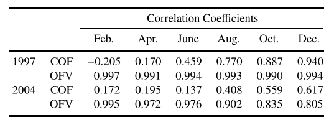
Table 1.Correlation coefficients of the observed versus simulated SST anomalies during the 1997 and 2004 El Niño years.OFV (COF)denotes the correlation coefficient of the SST anomalies simulated with OFV(COF)versus the observed anomalies.All results simulated with the OFV are statistically significant at the 99%confidence level.

Next,the OFV and COF(Fig.4)approaches in the simulations of the 2004 CP-El Niño event are compared(Fig.5). As pointedoutbyDuanet al.(2014),this El Niñoeventcould hardly be reproduced without the introduction of OFV.Table 1 lists the spatial correlations of the observed versus simulated SST anomalycomponentsduringthis El Niñoyear.The SST anomalies inthe spatial patterns simulatedwith OFV are very highly correlated with the observed patterns,whereas those simulated with COF are less correlated with the observations.Moreover,from its appearance,the 2004 event simulated by COF is hardly distinguishable as CP-El Niño or EP-El Niño,which is a critical factor to justify the simulation appearance.Considering that subsurface feedback may rarely affect the evolution of CP-El Niño(Kao and Yu,2009; Kug et al.,2009;Yu and Kim,2010;Duan et al.,2014),the OFV-corrected Zebiak–Cane model may not describe the observed thermocline depth variation,although it reproduces the SSTA component of CP-El Niño events well(Duan et al.,2014).This result can also be explained by the accompanying air–sea variables in the 2004 CP-El Niño simulated with COF.The seesaw pattern in the thermocline depth fields(Fig.3)and the slight eastward propagationof the zonal wind anomalies(Fig.2)differ from the observations,muddling the classification of the event(which evolves similarly to an EPEl Niño).

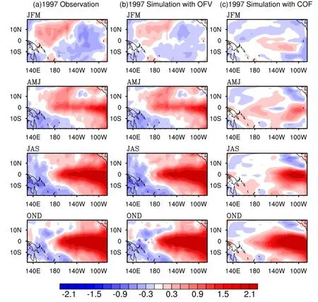
Fig.1.The SST anomaly(units:K)component of the seasonal evolutions of the observed 1997 El Niño event(a)and its simulations by the Zebiak–Cane model with OFV(b)and with COF(c).Here,a year is divided into four seasons: January to March(JFM),April to June(AMJ),July to September(JAS),and October to December(OND).

All of these results show that the OFV approach effectively offsets the time-variant model errors,which are better than those handled by COF.Corrected by the OFV method, the Zebiak–Cane model properly reproduces the El Niño events and improves the fit between the simulations and observations.In the COF approach,the model better simulated the 1997 El Niño than the 2004 El Niño.We also tested other El Niño events with the two approaches,as in Duan et al.(2014),and the comparison of COF and OFV changed little.That is,the model correction always performed better in EP-El Niño simulations than in CP-El Niño simulations,regardless of whether OFV or COF was adopted,and both the COF and OFV approach could further improve the simulation of EP-El Niño.In contrast,the time-dependent errors in the Zebiak–Cane model are particularly severe in CP-El Niño simulations,and the OFV rather than the COF approach could help reproduce a clear classification of the warm events.

3.3.Difference between COF and OFV

So why do bothapproacheshelp to reproducethe 1997El Niño event,while for the 2004 El Niño event the simulation benefits greatly from the OFV approach only?The differences between COF and OFV for the 2004 CP-El Niño may help to explain.

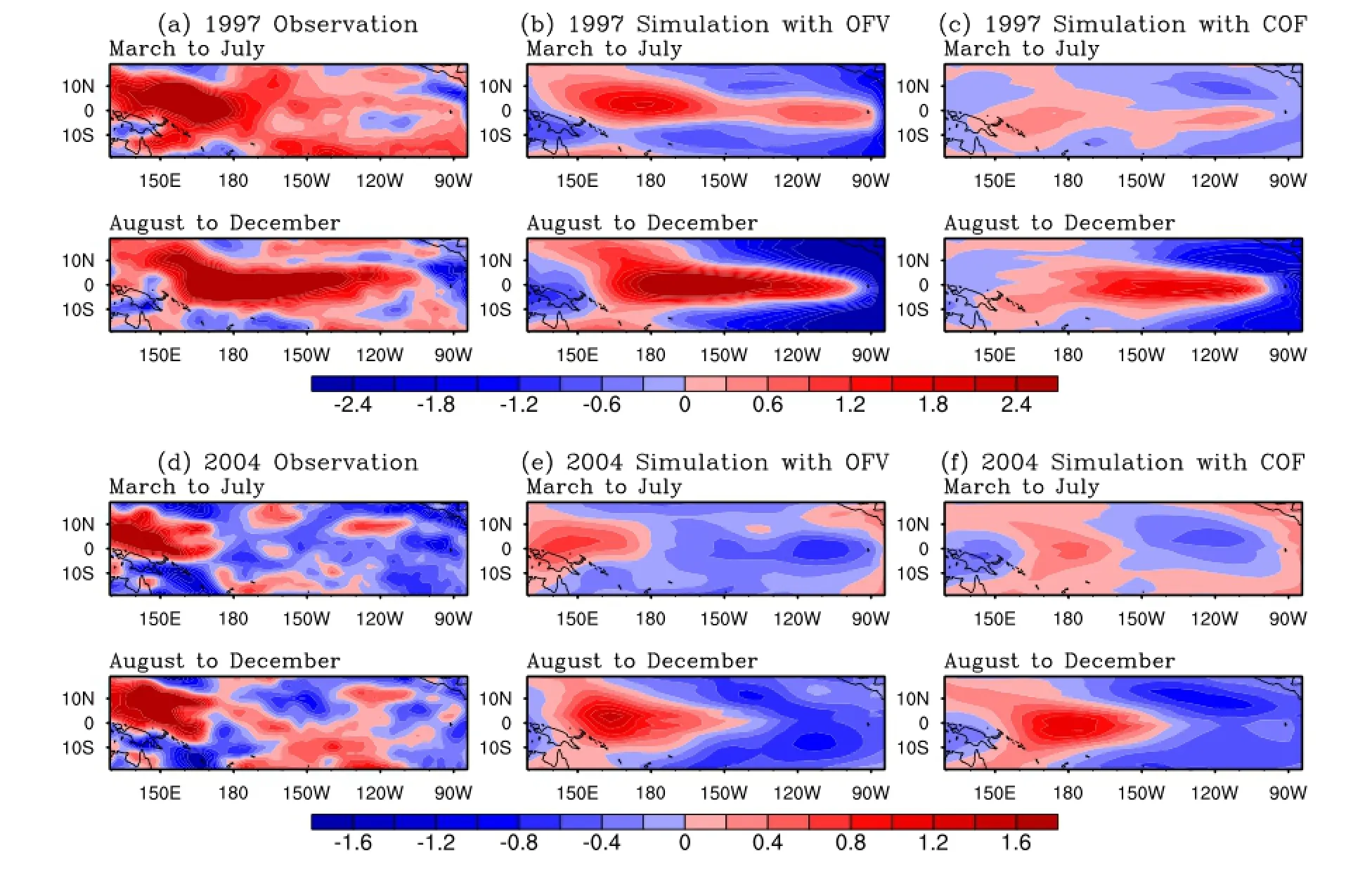
Fig.2.The zonal wind anomalies(units:m s-1)in the 1997 El Niño event.The anomalies are averaged from March to July and from August to December.(a)Observed zonal wind,derived from the NCEP–NCAR reanalysis data;(b) zonal wind simulated with OFV;and(c)zonal wind simulated with COF.Panels(d–f)show the corresponding results for the 2004 El Niño event.

Fig.3.As in Fig.2 but showing the thermocline depth anomalies(units:m).The observations are obtained from the EMC/CMB data.

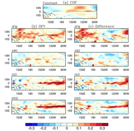
Fig.4.(a)COF and(b)OFV simulations(units:K month-1)of the 2004 El Niño event,and(c)their seasonal differences(OFV minus COF).The OFV includes 11 components in the El Niño year,corresponding to 11 time intervals (where one interval ranges from one month to the next).The COF includes a single component that remains constant throughout the year.

Specifically,in the 2004 El Niño,both the COF and OFV corrections yielded large positive values in the eastern tropical Pacific,suggesting that the uncertainties in the Zebiak–Cane model are dominated by SST tendency errors in this zone(Fig.4).On the other hand,seasonal differences between OFV and COF are apparent over the one-year evolution period.Throughout the first season,the uncertainties in the SSTA tendency traverse the entire tropical Pacific(Fig. 4b)in the OFV simulations but are lost in the western Pacific in the COF simulations.During spring(April–June),the differential plots(OFV-COF plots;see Fig.4c)exhibit limited regions of negative values in the eastern Pacific.In this season,it is apparent that the intensity of OFV is much weaker than at other times,while it helps to maintain the zonal gradient of SSTA fields(Fig.5b).In the latter half of the year,the positive values of COF are much smaller and the differences between OFV and COF cluster around the equator,particularly in the central-eastern Pacific(Figs.4b and c).Considering the SSTA growth rates related to OFV are nearly the same in the central and eastern Pacific in the latter half of the year(Fig.4b),the zonal gradient of SSTA evolution(Fig.5b) remains and helps concentrate warm water westward.Consequently,the SSTA increase in the equatorial central-eastern Pacific follows the zonal gradient of the SSTA field in the same area,favoring the westward march of the warm center from the Pacific east coast(Figs.5b and c).

3.4.Simulations by the OFV approach with different time intervals

Fig.5.The SST anomaly(units:K)component of the seasonal evolutions of the observed 2004 El Niño event(a)and its simulations by the Zebiak–Cane model with OFV(b)and with COF(c).

As described in section 2,the model error effects are offset by a proper time-variant external forcing f(x，t)that matches the simulations with the observations.To cope with the time-variant errors,the OFV method consists of several components within the time window[t0，tk]of the El Niño simulation.Selecting the intervalbetweeneachof these components is largely subjective but is important for reducingthe computationaltime of the simulations.In the simple Zebiak– Cane model,the time interval can be set to one or several months without affecting the computation.However,when the model tendency errors are offset by the OFV approach concerning a much more complicated model,the computational time may become unacceptable under the calculation conditions.On the one hand,extending the time interval of each OFV component reduces the cost of obtaining the OFV. On the other hand,adopting different time intervals for the OFV components and the different amount of observational data required consequently obscures the simulation performance.

Within the time window[t0，tk]of the OFV(see section 2),we selected time intervals of 1,2 and 3 months prior to the peak phase of the El Niño events for the OFV components(the 1-month interval was adopted in section 3.2). Giventhe predeterminedinitial anomalyfields and these simulationtime windows,we computedoneOFV componentevery month,every second month(January,March,May,July, September,November,December),and every third month (January,April,July,October,December),obtaining OFVs with 11 components,6 components and 4 components,respectively.For simplicity,we refer to these El Niño simulations as OFV,S-OFV and T-OFV,respectively.

To compare the SSTA evolutions simulated by OFV,we ran the Zebiak–Cane model forced by the corresponding SOFV and T-OFV for one year,obtained the simulations of both El Niño events,and checked their differences.The overall evolution features of the 1997 EP-El Niño event(Fig.6) are reproduced in both S-OFV and T-OFV,although the simulations differ slightly fromobservationsin the first season of the year.That is,the overall performances of S-OFV and TOFV are comparable to that of OFV.Similar conclusions can be drawn for the 2004 CP-El Niño(Fig.7).Central warming is observed even in the T-OFV simulation(three-month interval),and the SSTA pattern improves during the latter half of the year(see Table 2),indicating that the OFV-correctedZebiak–Cane model can reasonably simulate the 1997 and 2004 El Niño events at reduced computational cost.

Fig.6.The SST anomaly(units:K)components of the seasonal evolutions of the 1997 El Niño event simulated by the Zebiak–Cane model with(a)OFV,(b)S-OFV and(c)T-OFV,respectively.

Table 2.Correlation coefficients of the observed versus OFV-simulated SST anomalies in the 1997 and 2004 El Niño years. OFV(S-OFV,T-OFV)denote the correlation coefficients of the SST anomalies simulated with OFV(S-OFV,T-OFV)versus the observed anomalies.All results simulated with the OFV are statistically significant at the 99%confidence level.

Typically,as the model becomes more complicated,the integrations consume increasing amounts of time,regardless of finding the optimal forcing(OFV)for the tendency equation.We found that reducing the input of observational data(and hence the computational time)improved the costeffectiveness of the Zebiak–Cane simulations.Such cost reductions would benefit the OFV approach in more complicated CGCMs.

4.Conclusion and discussion

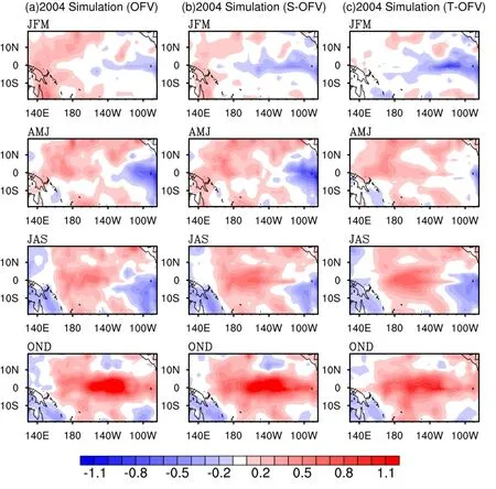
Fig.7.As in Fig.6 but simulating the 2004 El Niño.

Model errors are generally time-dynamic;therefore,an error-cancelation method that treats time-variant errors can potentially improve model simulations and predictions.In this study,ENSO simulations by the Zebiak–Cane model were corrected by COF and OFV,and the performances of the corrections were compared.The 1997 and 2004 El Niño events,which were badly reproduced by the uncorrected Zebiak–Canemodel to some extent,were better simulated by OFV and COF.But,nonetheless,it was found that the COF correction yields worse fits to El Niño observations comparedwith the OFV results,mainly because the latter handles time-variant model errors better.Specifically,when the initial anomalies were generated by couplingthe observed wind forcingtotheoceancomponent,theZebiak–Canemodelwith COF roughly reproduced the 1997 El Niño event;however, the 2004 El Niño simulated by COF defied an ENSO classification and the simulated evolution(warm SST concentrating in the central-eastern Pacific)typified an EP-El Niño event. Furthermore,the OFV approach effectively corrects the El Niño simulation model even when the observational data input(and thus the computational time)is reduced.This costeffective offset of model errors will favor the OFV approach in more complicated CGCMs.

Regarding the 2004 El Niño event,the differences in the SSTA patternsobtainedbyOFV andCOF revealedmanyseasonalvariations.Signalsof positiveSSTA tendencyprevailed in thewesternPacific at thebeginningofthe year;in thelatter half,positive anomalies were concentrated in the equatorial central-eastern Pacific(see Fig.4).Therefore,in this event, the SST tendency errors(which dominate the uncertainties in the Zebiak–Cane model)reflect the time-varying characteristics of the model errors.Furthermore,although the same SSTA growth rate introduced by OFV occurs in the central and eastern Pacific during the latter half-year,the warmer background to the west helps to generate stronger feedbacks between SSTAs and wind fields,and favors westward warming from the east coast of the Pacific.Consequently,the 2004 event appears as a CP-El Niño rather than an EP-El Niño.

In ENSO simulations,the multi-model mean state does not significantly change from CMIP3 to CMIP5,highlighting the potential for model error cancelation(Guilyardiet al., 2012).CP-El Niño simulations are particularly challenged by new feedback(which amplifies biases in the model),uncertain model parameters,and subjective contact with obser-vational data.The present paper proposes an efficient OFV application for model error treatment.Meanwhile,if we consider additionaltendencyequations of different physical variables including the SSTA equation,the performance of the approach might be further improved.Furthermore,it is necessary to introduce complicated models concerning ENSO simulations,which will properly benefit from the OFV approach.

Acknowledgements.This work was jointly sponsored by the National Basic Research Program of China(Grant No.2012CB 955202),the National Public Benefit(Meteorology)Research Foundation of China(Grant No.GYHY201306018),and the National Natural Science Foundation of China(Grant Nos.41176013 and 41230420).

REFERENCES

An,S.I.,and F.F.Jin,2001:Collective role of thermocline and zonal advective feedbacks in the ENSO mode.J.Climate, 14(16),3421–3432.

Ashok,K.,S.K.Behera,S.A.Rao,H.Y.Weng,and T.Yamagata,2007:El Niño Modoki and its possible teleconnection. J.Geophys.Res.,112,C11007,doi:10.1029/2006JC003798.

Barkmeijer,J.,T.Iversen,and T.N.Palmer,2003:Forcing singular vectors and other sensitive model structures.Quart.J.Roy. Meteor.Soc.,129(592),2401–2423.

Barreiro,M.,and P.Chang,2004:A linear tendency correction technique forimproving seasonal prediction ofSST.Geophys. Res.Lett.,31(23),L23209,doi:10.1029/2004gl021148.

Behringer,D.W.,M.Ji,and A.Leetmaa,1998:An improved coupled model for ENSO prediction and implications for ocean initialization.Part I:The ocean data assimilation system.Mon.Wea.Rev.,126(4),1013–1021.

Blumenthal,M.B.,1991:Predictability of a coupled oceanatmosphere model.J.Climate,4(8),766–784.

Bourassa,M.A.,Rosario Romero,Shawn R.Smith,and James J. O’Brien,2005:A new FSU winds climatology.J.Climate, 18,3686–3698,doi:http://dx.doi.org/10.1175/JCLI3487.1.

Chen,D.K.,S.E.Zebiak,A.J.Busalacchi,and M.A.Cane,1995: An improved procedure for El Niño forecasting:Implications for predictability.Science,269,1699–1702.

Chen,D.K.,C.M.Cane,S.E.Zebiak,R.Cañizares,and A.Kaplan,2000:Bias correction of an ocean-atmosphere coupled model.Geophys.Res.Lett.,27(16),2585–2588,doi:10.1029/ 1999gl011078.

Chen,D.K.,M.A.Cane,A.Kaplan,S.E.Zebiak,and D.J.Huang, 2004:Predictability of El Niño over the past 148 years.Nature,428(6984),733–736.

D’andrea,F.,and R.Vautard,2000:Reducing systematic errors by empirically correcting model errors.Tellus A,52(1),21–41.

Duan,W.S.,B.Tian,and H.Xu,2014:Simulations of two types of El Niño events by an optimal forcing vector approach.Climate Dyn.,43,1677–1692,doi:10.1007/s00382-013-1993-4.

Evensen,G.,1994:Sequential data assimilation with a nonlinear quasi-geostrophic model using Monte Carlo methods to forecast error statistics.J.Geophys.Res.,99(C5),10 143–10 162.

Feng,F.,and W.S.Duan,2013:The role of constant optimal forcing in correcting forecast models.Science China Earth Sciences,56(3),434–443.

Guilyardi,E.,H.Bellenger,M.Collins,S.Ferrett,W.J.Cai,and A.T.Wittenberg,2012:A first look at ENSO in CMIP5.CLIVAR Exchange,17,29–32.

Ham,Y.G.,and J.S.Kug,2012:How well do current climate models simulate two types of El Niño?Climate Dyn.,39(1–2),383–398,doi:10.1007/s00382-011-1157-3.

Kalnay,E.,and Coauthors,1996:The NCEP/NCAR 40-year reanalysis project.Bull.Amer.Meteor.Soc.,77(3),437–471.

Kao,H.Y.,and J.Y.Yu,2009:Contrasting eastern-Pacific and central-Pacific types of ENSO.J.Climate,22(3),615–632.

Kim,S.T.,J.Y.Yu,A.Kumar,and H.Wang,2012:Examination of the two types of ENSO in the NCEP CFS model and its extratropical associations.Mon.Wea.Rev.,140(6),1908–1923.

Kug,J.S.,F.F.Jin,and S.I.An,2009:Two types of El Niño events:Cold tongue El Niño and warm pool El Niño.J.Climate,22(6),1499–1515.

Kug,J.S.,J.Choi,S.I.An,F.F.Jin,and A.T.Wittenberg,2010: Warm pool and cold tongue El Niño events as simulated by the GFDL 2.1 coupled GCM.J.Climate,23(5),1226–1239.

Leith,C.E.,1978:Objective methods for weather prediction. Annual Review of Fluid Mechanics,10(1),107–128,doi: 10.1146/annurev.fl.10.010178.000543.

Lorenz,E.N.,1965:A study of the predictability of a 28-variable atmospheric model.Tellus,17(3),321–333.

Morss,R.E.,K.A.Emanuel,and C.Snyder,2001:Idealized adaptive observation strategies for improving numerical weather prediction.J.Atmos.Sci.,58(2),210–232.

Mu,M.,W.S.Duan,and B.Wang,2003:Conditional nonlinear optimal perturbation and its applications.Nonlinear Processes in Geophysics,10(6),493–501.

Rayner,N.A.,D.E.Parker,E.B.Horton,C.K.Folland,L. V.Alexander,D.P.Rowell,E.C.Kent,and A.Kaplan, 2003:Global analyses of sea surface temperature,sea ice, and night marine airtemperature since the latenineteenth century.J.Geophys.Res.,108(D14),4407,doi:10.1029/2002JD 002670.

Roads,J.O.,1987:Predictability in the extended range.J.Atmos. Sci.,44(23),3495–3527.

Talagrand,O.,1997:Assimilation of observations,an introduction.J.Meteor.Soc.Japan,75,191–209.

Tang,Y.M.,Z.W.Deng,X.B.Zhou,Y.J.Cheng,and D.K.Chen, 2008:Interdecadal variation of ENSO predictability in multiple models.J.Climate,21(18),4811–4833.

Toth,Z.,and E.Kalnay,1997:Ensemble forecasting at NCEP and the breeding method.Mon.Wea.Rev.,125(12),3297–3319.

Vannitsem,S.,and Z.Toth,2002:Short-term dynamics of model errors.J.Atmos.Sci.,59(17),2594–2604.

Xue,Y.,M.A.Cane,S.E.Zebiak,and M.B.Blumenthal,1994: On the prediction of ENSO:A study with a low-order Markov model.Tellus A,46(4),512–528.

Yu,J.Y.,and S.T.Kim,2010:Three evolution patterns of central-Pacific El Niño.Geophys.Res.Lett.,37,L08706,doi: 10.1029/2010GL042810.

Zebiak,S.E.,and M.A.Cane,1987:A model El Niño-southern oscillation.Mon.Wea.Rev.,115(10),2262–2278.

Tian,B.,and W.S.Duan,2016:Comparison of constant and time-variant optimal forcing approaches in El Niño simulations by using the Zebiak–Cane model.Adv.Atmos.Sci.,33(6),685–694,

10.1007/s00376-015-5174-8.

29 July 2015;revised 15 November 2015;accepted 21 December 2015)

Wansuo DUAN

Email:duanws@lasg.iap.ac.cn