Numerical Simulation of Large Scale Structures andCompressibility Effect in Compressible Mixing Layerswith a Discontinuous Galerkin Method

Xiaotian Shi, Wei Wang, Guiru Zhang, Tiejin Wang, Chi-wang Shu

(1. China Academy of Aerospace Aerodynamics, Beijing 100074, China 2. Brown University, Providence RI 02912, USA)



Numerical Simulation of Large Scale Structures andCompressibility Effect in Compressible Mixing Layerswith a Discontinuous Galerkin Method

Xiaotian Shi1,*, Wei Wang1, Guiru Zhang1, Tiejin Wang1, Chi-wang Shu2

(1. China Academy of Aerospace Aerodynamics, Beijing 100074, China 2. Brown University, Providence RI 02912, USA)

Large scale structures in two or three dimensional spatially developing compressible mixing layers, as well as compressibility effect in supersonic mixing layers under the convective Mach numberMc=0.4 andMc=0.8 respectively are numerical studied with a discontinuous Galerkin method. Special attention is paid on the panorama of spatial evolution of large scale structures and the compressibility effect. Theλ2structureextractionmethodisutilizedinthispaper,the“forest”structuresareevident.TheturbulenceandReynoldsstressofthemixinglayersarefounddecreasingwithMcin current simulations, which is expected to offer useful guidance for turbulent modeling in RANS and LES. The current study also shows the success of discontinuous Galerkin method to do compressible turbulence simulation.

Discontinuous Galerkin Method, Supersonic mixing layers, Large scale structures, Compressibility effects

Numenclature

Mc=convective Mach number

ρ=density

a=speed of sound

p=pressure

e=internal energy

Cv=specific heat at constant volume

γ=ratio of specific heat

0 Introduction

Structure evolution and compressibility effect are two unfading topics in compressible mixing layers study, and it is believed that the compressibility effect affect the behavior of structures and then further affect on the growth rate of mixing layers, so it is meaningful to investigate the behavior and the evolution of large scale structures with compressibility effect in compressible mixing layers.

CFD is a powerful tool to do compressible mixing layers study, take the numerical work of [1-7] as examples. However, it should be pointed out that most of the numerical work concern temporal developing mixing layers for computational load consideration, which is useful to investigate the time evolution of structures but can not gain the spatial evolution of structures and transition characteristic of the flow.As for spatially developing compressible mixing layers, the knowledge of large scale coherent structures evolution is still too limited and premature. Actually, good simulation of vortex and shock structures is not an easy task of numerical schemes. Discontinuous Galerkin (DG) finite element method, greatly developed by [8,9], is a high resolution numerical method with the ability of high order accuracy and good discontinuous capture ability, it has low numerical dissipation and easy to be parallel programmed, these advantages make it very suitable for compressible flow simulation and very popular up to date. Shi [10] successfully did direct numerical simulations of two or three dimensional spatially developing compressible mixing layers with the DG scheme, fairly well results were obtained. The spatial evolution of large scale structures, both in two and three dimensions, were visualized and investigated in detail, as well as the characteristics of transition and passive scalar field.

To visualize large scale structures, people prefer to vorticity and pressure fields for two dimensional cases, but it is not a trivial thing for three dimensional cases. There are several structures definition methods for three dimensional complex flow, such as vorticity magnitude |ω|,λ2andQ2method. |ω| has been widely used in early time to educe coherent structures, but may not always be satisfied since it does not identify vortex core in a shear flow.λ2is the second largest eigenvalue of the symmetric tensor ofS2+Ω2[11], whereSandΩare the symmetric and the anti-symmetric components of the velocity gradient tensor. Ifλ1≥λ2≥λ3aretheeigenvaluesofS2+Ω2,λ2-definitionisequivalenttotherequirementthatλ2<0withinthevortexcore.Theλ2-definitioncorrespondstothepressureminimuminaplaneandonlythecontributionofS2+Ω2top,ijistakenintoaccount.preferλ2isbettertoeducecoherentstructures,moreinformationcanbefoundinreference.Hereinthispaper,λ2methodisusedtoextractlargescalestructures.

ThepurposeofthispaperistoshowtheprocessofsolvingNSequationwithDiscontinuousGalerkinmethodindetail,andshowthesuccessofDGonfreeshearturbulencesimulation.Furthermore,thewholeviewofspatialevolutionoflargescalestructuresintwoorthreedimensionalspatiallydevelopingcompressiblemixinglayersispresented,exhibitingthecompressibilityeffectonstructuresandtheircharacteristicsduringtransitionprocess.

1 Optimization Framework

1.1 Governing Equations

For the full three dimensional compressible Navier-Stokes (N-S) equations, the non-dimensional form are,

(1)

wheretheconservevariablesuand Euler fluxesFe=(f1(u),f2(u),f3(u))are

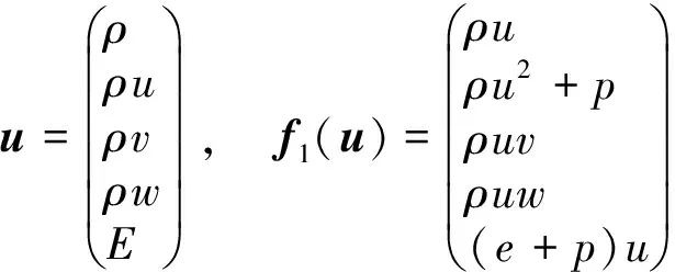
(2)

(3)

(4)

And

(5)

respectively. WhereμisphysicalviscositybySutherlandlawandλ=-2μ/3thesecondviscositycoefficientwith“Stokesassumption”,andPrisPrandtlnumber. (),x, (),yand(),zarederivativesofphysicalvariableswithrespecttothethreecoordinatecomponents.Thenon-dimensionalparametersinthegoverningequationsareMa,Re,Pr,γ.

1.2 DG Discretization

1.2.1 Euler Equation

For simplicity, we assume that the calculation domainΩis a collection of rectangle cellJh,andfortwoelementsK1andK2,ife=K1∩K2≠Ø,theneis either an edge of bothK1andK2orapoint.WedenotebyVhthepolynomialspacewiththeordernotlargerthanpndefinedonK∈Jh.WemultiplytheEulerequationbyatestfunctionvh∈VhandintegrateoverK∈Jh,replacetheexactsolutionuby its approximationuh∈Vh,thereis:

-∫KFe(uh)·vhdK=0

∫Kuh(t=0)vhdK=∫Ku0vhdK, ∀vh∈Vh

(6)

Inoursimulation,thebasisfunctionischosenasLegendrepolynomial

(7)

Atthecellboundary,thenumericalfluxisobtainedbylocalLax-Friedrichs fluxes. For time advance, third order accuracy Runge-Kutta is used.

1.2.2 N-S Equation

The gradients of velocityS=u[12]inviscosityfluxesisincludedasanewvariabletoreducetheorderofthepartialdifferentialequations(PDE)

S-u=0

(8)

ut+·F(u,S)=0

(9)

DiscretizingthecomputationaldomainΩas a collection of non-overlapping brick elementsK, multiplying the PDE with “test function”qandw, integrating them by parts on each cell, we obtain the weighted residual formulation of N-S equations

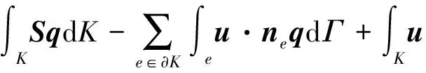
(10)

-∫KFe(u)·

(11)

Oneachelement,taketheplaceofu,S,q,win Eq.(10) and (11) by their projection uh, Sh, qh, whinthepolynomialspaceVhwiththeordernomorethank

(12)

1.2.3DiscontinuousIndicator

TherearetwokindsoflimiterinRK-DGcalculation,namelyTVD(TotalVariationDiminishing)andTVB(TotalVariationBounded)limiter.TVDlimiterhaslargerdissipationthanaTVBlimiter.Inoursimulation,adiscontinuousindicatorfromWENOisused[13]tokeephighresolutionbothonsmoothandstrongdiscontinuouszones.

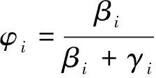
αi=|ui-1-ui|2+ε,

ξi=|ui-1-ui+1|2+ε,

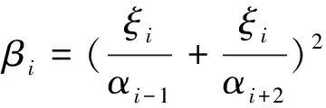
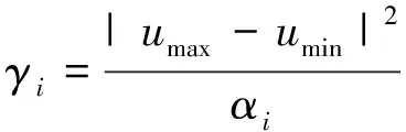
(13)

Theindicatortakesthevalue0asstrongdiscontinuousoccurredand1insmoothzones.ThentheTVBlimiterconstantisaconstantmultiplythediscontinuousindicator.

(14)

Inthismanner,theschemecankeephighresolutioninthecalculationdomain.

1.2.4TestCases

Shu-Osher Test Problem

Shu-Osher test problem [14] is a one dimensional problem that reflects interaction between wave and shock structures, the Euler equation is solved with initial condition

(15)

and third-order accuracy, both with TVD and TVB limiter. The space step is Δx= 1/40, TVB constant isM=300 for TVB limiter. Numerical results are shown in Fig.1, from which we can see the advantage of DG scheme on detailed structures presentation, and a suitable TVB constant can improve the resolution significantly.

From figure 1, the P2 limiter with TVB constantM=300 “Proj4m300phi” is the best and ready for our mixing layer simulation.

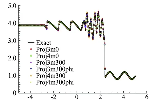
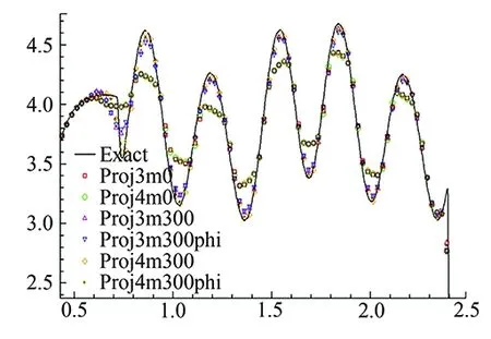
Fig.1 Simulation results and zoom in of Shu-Osher test program.

Forced N-S Equation

A Forced N-S equation which has exact solution as Eq.(16)

(16)

issolvedtovalidatethecodeforN-Sequation,thesimulationresultsisTable1,thirdorderaccuracyisobtainedforP2TVDRK-DG.

1.3 Computational Details

1.3.1 Run Conditions

The equation is solved with a third order accuracy DG scheme, Legendre polynomial is taken as the basis functions. The time marching is done with a third order Runge-Kutta method. The numerical mesh is uniform inxdirectionandstretchedfromthestreamsinterfacetooutsideinydirection,theparametersofcalculationdomainandgrids,aswellasflowparametersarelistedinTable2.

1.3.2GridFreeValidation

Figure2showsthegridvalidationofthecurrentschemeforthesimulationofcaseMc=0.4, where

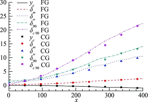
(a) Center of the mixing layer yc, momentum thickness δm, vorticity thickness δω, nominal thickness δ90

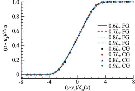
(b) Mean streamwise velocity comparison for different stream positions, the ycoordinate is normalized with δmFig.2 Numerical comparison of the results obtained with the coarse grid and the fine grid for the case Mc=0.4.

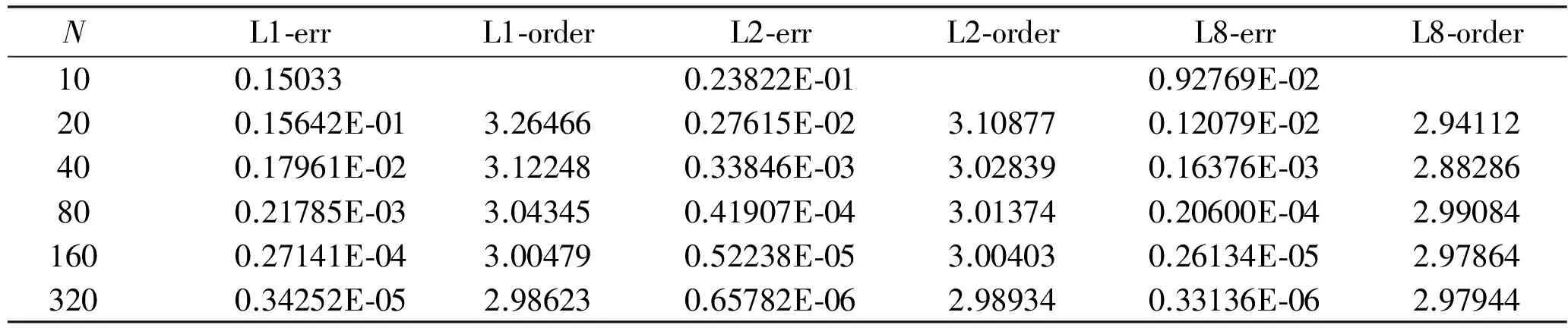
Table 1 Accuracy test of forced NS equation with P2 TVD RK-DG method

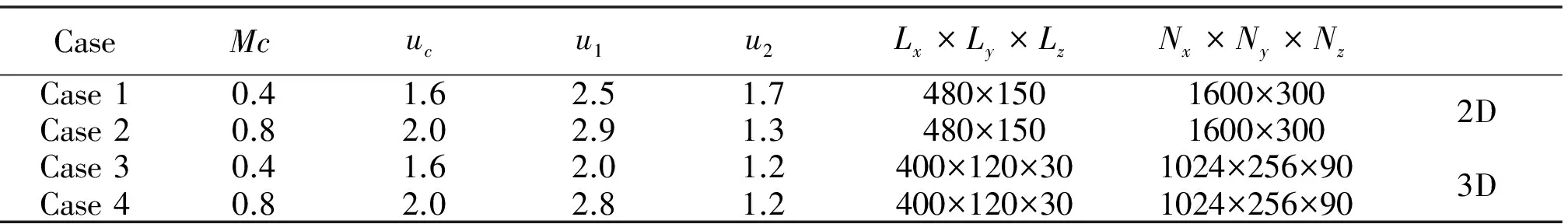
Tabel 2 Parameters of calculation domain and grids

2 Results and Discussion

2.1 Large Scale Structures Visualization

2.1.1 Two Dimensional Cases

Fig.3 shows the typical instantaneous results of the 2D spatially developing compressible mixing layers with the convective Mach numberMc=0.4andMc=0.8fromtheDNSresults.Fig.3 (a)showstheinstantaneouspressurefieldofcaseMc=0.4,fromwhichthesmallfinesonicwavesatthemixinglayersinletcanbeclearlyseen,thegreenlowpressurelocateinthecenterofvortexesandtheredhighvaluesbetweentwoneighborvortexes.Fig.3 (b)showstheconcentrationfield,fromwhichlargescalecoherentstructuresofBrown-Roshkovortexcanbeeasilyseen.Fig.3 (c)andFig.3 (d)showthepressureandconcentrationfieldsofcaseMc=0.8.FromFig.3,itcanbeseenthat,atupstream,theperturbationischosenbythefields,thesignalsnearthemostunstablefrequencybegintobeamplifiedandevaluatetolargescalestructures.Duetointeractionbetweenvortexesandshocklets,thefieldsbecomecomplexatdownstream.ThepassivescalarmixingisdominatedbylargescalestructuresforthelowerMccase. For the higherMccase, the phenomenon of “engulfing” can be seen at the position aboutx=350fromFig.3 (d),wheretheconcentrationisengulfedfromthehighspeedstreamtothelowspeedstreamwithoutmixingsufficiently.

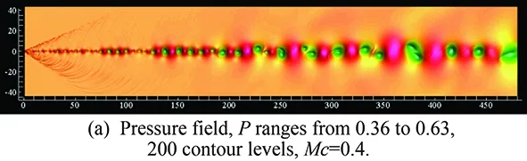
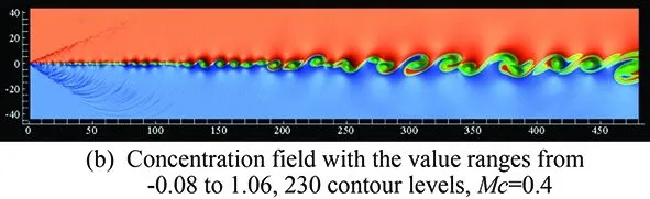
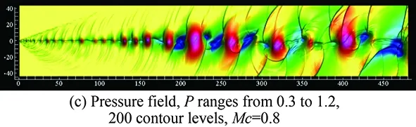
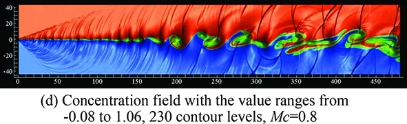
Fig.3 Large scale structures in the two-dimensional compressible mixing layers with the convective Mach number Mc=0.4 and Mc=0.8.

InthecaseMc=0.8,thetwodifferentthingstothelowerMccase are that strong shock waves appear due to the high compressibility effect and the vortex structures are flatted. Shocklets structures have been reported in the numerical work of [1,3,5,7,15] and experimental work of [16, 17]. Actually, shocklet structures have close relationship with large scale vortex. The orientation of shocklet structures is changed as the process of turnover of large scale vortex. Figure 4 shows the snapshots of instantaneous pressure field withMc=0.8atthetimet=1 782, 1 797, 1 812, 1 827,atypicaltwovortexmergingprocessiscoloredwithrectanglezones.Fromwhichwecanseethattheevolutionprocessissimilartothatoftemporaldevelopingmixinglayersforthecompressibilityeffect,apairofshockletsappearatupperanddownpartofavortex,theshockletsintheexpansionzonebecomeweakeranddisappear,whiletheshockletsincompressionzonebecomestrongerandsurvived.Intemporaldevelopingcases,theevolutionofshockletsismainlyaffectedbytwovortexesmergingforthereasonthatthecalculationdomainisingeneralevenintegertimesofperturbationwavelength.Whileinspatialdevelopingmixinglayers,theinteractionbetweenshockletsandvortexesbecomemorecomplexbecausethefieldcontainsricherfrequencyofperturbation,therandomvortexesmergingmakesthebehaviorofshockletsneartothenaturalhappenedmixinglayers.

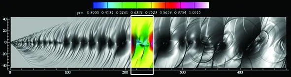
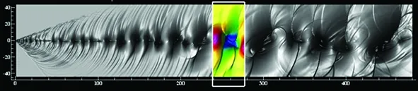
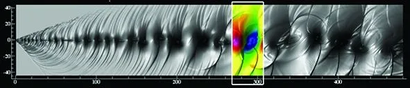
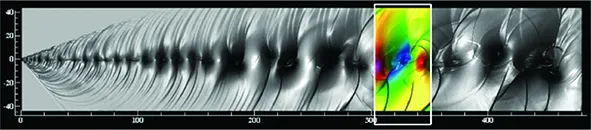
Fig.4 Snapshots of instantaneous pressure field with Mc=0.8 at the time t=1 782, 1 797, 1 812, 1 827, the colorful parts are typical evolution of two-vortex merging.

2.1.2ThreeDimensionalCases

Fig.5andFig.6givetheinstantaneousvisualizationoflargescalestructuresdefinedwiththeλ2method for casesMc=0.4 andMc=0.8, the color reflect the velocity value component in streamwise direction. At the slicez=0, equal pressure contour is plotted to visualize the expansion/compression waves.

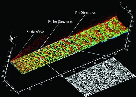
Fig.5 Large scale structures defined with λ2 method in 3D spatially developing compressible mixing layers with Mc=0.4,x ranges from -2 to 202, iso-surface of λ2=-0.001, colored with stream-wise velocity magnitudeU (1.2～2.0, 40 contour levels).

Fig.6 Large scale structures defined with λ2 method in 3D spatially developing compressible mixing layers with Mc=0.8,x ranges from -2 to 202, iso-surface of λ2=-0.008, colored with stream-wise velocity magnitudeU (1.2～2.8, 40 contour levels).

From Fig.5, we can see clearly the whole process of large scale structures evolution in the lowerMccase, which is similar to that of incompressible case. After chosen by the field, the perturbation signal added at the inlet is amplified in some frequencies. Well organized large scalerollerstructures begin to form for the two dimensional Kelvin-Helmholtz instability. With the developing, the second instability in the span-wise direction begins to work, which makes the two neighboring roller structures be connected by theribstructures. Theribsgrow in further downstream of the field, stream-wise vortexes with aλshapebegintoflourishandtheflowtransitsintofullydevelopedturbulence.FromtheLST,themostunstableperturbationsignalistwodimensionalinthiscase,nosignificantobliquemodeisobserved,andthemaininstabilityisinthestream-wisedirection.Thepressurefieldintheslicez=0revealsthatsonicwavestructureslocateattheinletofthefield,andexpansion/compressionwavestructuressetnearthelargescalestructures,nostrongdiscontinuousarefound.Fig.6showsustheevolutionoflargescalestructuresinthehigherMccase, it is different from caseMc=0.4∶1) the structures are finer and have smaller scale than that of the lowerMccase for the increasing three dimensional characteristic of structures, and it seems that the transition happens earlier. 2) Strong compressible wave structures appear for the increasing compressibility effects, as distinctly shown in the flood of pressure field in thezdirection slice. The forest of structures becomes flourishing downstream and the field becomes more complex.

2.2 Compressibility on Reynolds Stress

After a long time average, statistical results of the simulations are obtained, the mean flow has the self-similarity property downstream in density, pressure and velocity field, as well as turbulence and Reynolds stress.

Fig.7 gives the profiles of mean density and mean velocity component in cross flow direction at different stream-wise position for caseMc=0.4. The profiles at different stream position collapse toalmost a same curve in the coordinate ofξ=(y-yc(x))/δm(x),which means a good self-similarity property is obtained, it is a statistical characteristic of free shear flow and means that the current simulation is believable. Actually, not only the mean physical variables, such as pressure, velocity, temperature, but also the turbulence intensities are self-similar.

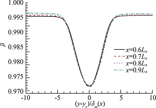
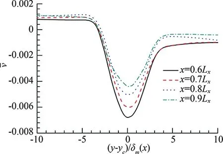
Fig.7 Self-similar of mean pressure for three dimensional case Mc=0.4, profiles at positionsx=0.6Lx, 0.7Lx, 0.8Lx, 0.9Lx, the coordinatey is scaled with local momentum thickness δm(x).

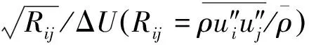
Fig.8 gives the average profiles of turbulence intensity components and Reynolds stress in self-similar region, the average is done along the coordinate ofξ. For convenience, results from experimental results [21,22], DNS results of [18,20], LES results of [21], are also plotted.

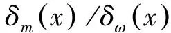
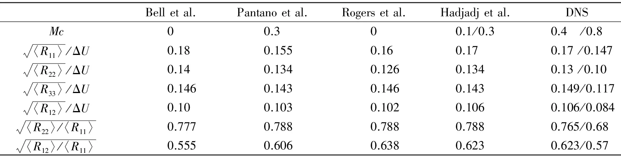
Table 3 Comparison of peak turbulent intensities of compressible mixing layers with references

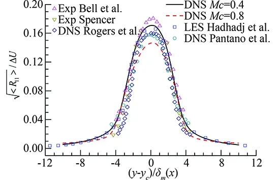
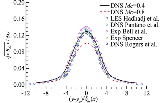
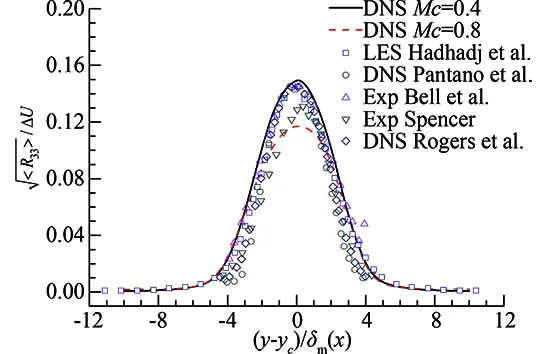
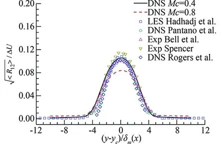
Fig.8 Turbulence intensity and Reynolds stress comparison for caseMc=0.4 andMc=0.8.

3 Conclusion and Future Work

The process of solving NS equation with TVD- or TVB-RK Discontinuous Galerkin method is given in this paper in detail. To low order the NS equation, an intermediate variableS=uis introduced and solved with the convection-diffusion PDE.

The simulation results of test cases show that the current code is credible and ready to do mixing layer simulations. Spatial developing mixing layers both in two dimensions and three dimensions are simulated with convective Mach numberMc=0.4 andMc=0.8.

Special attention is paid to the spatial evolution of large scale structures and compressibility effect both on structures and turbulence variables. The charac-teristic of large scale structures are fully demon-strated, which show the potential ability of DG on compressible free shear turbulence simulation.

Implicit time advancement and hybrid method of finite volume and DG will be the next step work in future, and the compressibility effect will be studied quantitatively.

[1]Lele S K, Direct numerical simulation of compressible free shear flows; AIAA 89-0374[R]. Reston: AIAA, 1989.

[2]Sarkar S. The stabilizing effect of compressibility in turbulent shear flow[J]. J. Fluid Mech., 1995, 282: 163-186.

[3]Vreman B. Direct and Large-eddy simulation of the compressible turbulent mixing layer[R]. University of Twente, Department of Applied Mathematics,Thesis, 1995.

[4]Vreman A, Sandham N, et al. Compressible mixing layer growth rate and turbulence characteristics[J].J. Fluid Mech., 1996. 320: 235-258.

[5]Freund J, Lele S, et al. Compressibility effects in a turbulent annular mixing layer. Part 1. Turbulence and growth rate[J].J. Fluid Mech., 2000, 421: 229-267.

[6]Freund J, Moin P, et al. Compressibility effects in a turbulent annular mixing layer. Part 2. Mixing of a passive scalar[J].

J. Fluid Mech., 2000, 421: 269-292.

[7]Li Q, Fu S. Numerical simulation of high-speed planar mixing layer[J]. Computers & Fluids. 2003,32(10):1357-1377.

[8]Cockburn B, Lin S Y, et al. TVB Runge-Kutta local projection discontinuous Galerkin finite element method for conservation laws III: one dimensional systems[J]. J. Comp. Phys., 1989, 84: 90-113.

[9]Cockburn B, Shu C-W. The Runge-Kutta discontinuous Galerkin method for conservation Laws: multidimensional systems. J. Comput. Phys, 1998,141(2): 199-224.

[10]Shi X T, Chen J, et al. Numerical simulations of compressible mixing layers with a discontinuous Galerkin method[J]. Acta Mechanica Sinica, 2019, 27(3): 318-329.

[11]Jeong J, Hussain F. On the identification of a vortex[J]. Journal of Fluid Mech., 285: 69-94.

[12]Bassi F, Rebay S.Numerical evaluation of two discontinuous Galerkin methods for the compressible Navier-Stokes equations[J]. Int. J. Numer. Meth. Fluids,2000, 40: 197-207.

[13]Xu Z, Shu C-W. Anti-diffusive flux corrections for high order finite difference WENO schemes[J]. J. Comp. Phys., 2005, 205: 458-485.

[14]Shu C-W, Osher S. Efficient implementation of essentially non-oscillatory shock-capturing schemes[J]. J. Comp. Phys., 1988. 77: 439-471.

[15]Fu D X, Ma Y W. Direct numerical simulation of coherent structures in planar mixing layer[J]. Science in China A, 1996, 26(7): 657-664.

[16]Papamoschou D, Roshko A. The compressible turbulent shear layer: an experimental study[J]. J. Fluid Mech., 1988, 197: 453-477.

[17]Clemens N T, Mungal M G. Large-scale structure and entrainment in the supersonic mixing layer[J]. J. Fluid Mech., 1995, 284:171-216.

[18]Rogers M M, Moser R D. Direct simulation of a self-smilar turbulent mixing layer[J. Phys. Fluids, 1994,6(2): 903-923.

[19]Bell J, Mehta R. Development of a two-stream mixing layer from tripped and untripped boundary layers[J]. AIAA Journal, 1990,28(12):2034-2042.

[20]Pantano C, Sarkar S. A study of compressibility effects in the high-speed turbulent shear layer using direct simulation[J]. J. Fluid Mech., 2002,451.

[21]Hadjadj A, Yee H C, Sjogreen B. LES of temporally evolving mixing layers by an eighth-order filter scheme[J]. Int. J. Num. Meth. in Fluids. 2012, 70(11): 1405-27.

[22]Spencer B W, Jones B. Statistical investigation of pressure and velocity fields in the turbulent two-stream mixing layer; AIAA-71613[R]. Reston: AIAA, 1971.

0258-1825(2016)02-0224-08

基于间断有限元方法的可压缩混合层中大尺度结构和压缩性效应的数值模拟研究

时晓天1,*，王 伟1， 张桂茹1，王铁进1，舒其望2

(1. 中国航天空气动力技术研究院， 北京 100074, 中国; 2. 布朗大学，罗得岛州 普罗维登斯市 02912, 美国)

基于间断有限元方法(DGM)，对二维和三维、对流马赫数Mc=0.4和0.8的空间发展的可压缩混合层进行了数值模拟，并对混合层中的大尺度结构及压缩性效应进行了研究。重点观察了大尺度结构随压缩性变化的全景图像，文中采用λ2方法定义三维流动中的大尺度结构，流场中能够观察到大尺度的涡结构森林。当前数值模拟表明混合层的湍动能和雷诺应力随对流马赫数的增加而降低，这对RANS和LES模型的建立具有一定的参考意义。本研究也表明，间断有限元方法能够成功地应用于可压缩湍流的数值模拟。

间断有限元方法;超声速混合层;大尺度结构;压缩性效应

V211.3

A doi: 10.7638/kqdlxxb-2016.0004

*Assistant Professor;xxtshi@163.com

format: Shi X T, Wang W, Zhang G R, et al. Numerical Simulation of Large Scale Structures and Compressibility Effect in Compressible Mixing Layers with a Discontinuous Galerkin Method[J]. Acta Aerodynamica Sinica, 2016, 34(2): 224-231.

10.7638/kqdlxxb-2016.0004. 时晓天,王伟,张桂茹,等. 基于间断有限元方法的可压缩混合层中大尺度结构和压缩性效应的数值模拟研究(英文)[J]. 空气动力学学报, 2016, 34(2): 224-231.

Received： 2015-12-15; Revised：2016-01-10

Supported by the National Natural Science Foundation (No.11302213)