An ef ficient latent variable optimization approach with stochastic constraints for complex industrial process☆

Zhengshun Fei*,Kangling Liu ,Bin Hu ,Jun Liang

1 School of Automation and Electrical Engineering,Zhejiang University of Science and Technology,Hangzhou 310023,China

2 State Key Lab of Industrial Control Technology,Institute of Industrial Control Technology,Department of Control Science and Engineering,Zhejiang University,Hangzhou 310027,China

3 Department of Electrical Engineering,University of Notre Dame,Notre Dame,IN 46556,USA

Keywords:Data-driven model Optimization Partial least square Polymerization

ABSTRACT For complex chemical processes,process optimization is usually performed on causal models from first principle models.When the mechanism models cannot be obtained easily,restricted model built by process data is used for dynamic process optimization.A new strategy is proposed for complex process optimization,in which latent variables are used as decision variables and statistics is used to describe constraints.As the constraint condition will be more complex by projecting the original variable to latent space,Hotelling T2 statistics is introduced for constraint formulation in latent space.In this way,the constraint is simpli fied when the optimization is solved in low-dimensional space of latent variable.The validity of the methodology is illustrated in pH-level optimal control process and practical polypropylene grade transition process.

1.Introduction

Modern industrialprocess is becoming more and more complex and its operation needs optimization to improve system performance.For complex process systems with dynamic,nonlinear and multiple-state characteristics,process optimization often relies on process models.The first-principle model is commonly used in process optimization.For most practical processes,developing first-principle models is dif ficult and time-consuming.Therefore,simpli fied data-driven models are usually used as an alternative[1,2]and restricted modelbuiltby process data is used for process optimization.A great number of process variables exist in most complex processes and are often correlative.In such cases,latent variable based approach such as partial least squares(PLS)[3]is often used to model the process with relative historical operating data.It is quite important to develop a data-based optimization approach that can optimize complex process easily.

Attemptshave been made to use PLS latentvariable approach in process optimization and quality design[4,5].A methodology is developed for process development and control based on optimization in the subspace de fined by latentvariable models[6],in which optimization problem is formulated with solutions restricted in the latent variable space with the model de fined by training data set.Jaeckle and MacGregor[7]have proposed a latentvariable approach to estimate operating conditions in order to yield a final productwith desired quality characteristics,with the empiricallatentvariable models fitted to historicalprocess data.The methodology is extended to estimate time-varying pro files of manipulated variables for batch process by developing an optimization framework[8,9]and the constraints of process operating trajectories are also considered[10].As the optimization is easier in the lowdimensional space of latent variables,latent variable method can be used to develop robust processes[11]and to design model predictive control(MPC)strategy.For batch[12-14]and continuous[15,16]processes,the control problem can be solved in the low-dimensional latent variable space to obtain MPC methodologies.In most of these studies,justthe static optimization has been considered based on latentvariable approach,while dynamic behavior is commonly present in practical processes.

In this work,complex industrial processes are optimized in latent space and latentvariables are used as decision variables in optimization.The PLS based latent variable modeling methodology is introduced,in which polynomial cascaded ARX inner model structure is used for modeling nonlinear and dynamic process with historical operating data.With latent variables as optimization variables,higher dimension of original variables is reduced to lower dimension of latent variables,so the computing burden will be lightened.The optimization can easily be performed in the low-dimension space of latent variables even though the number of process variables is quite large.The Hotelling T2statistics constraint is used in the optimization model.The developed approach is first illustrated with a pH optimal control process and then applied in practical polypropylene grade transition process.The computing burden in latent variable space for dynamic optimization will be reduced and the constraint condition will be simpli fied by using Hotelling T2statistics.

2.PLS Latent Variable Modeling

2.1.Dynamic nonlinear PLS model structure

Partialleast squares(PLS)[17,18],also known as projection to latent structures,is a latent-variable based method for modeling the relationship between a setof predictor variables and a set of response variables.Before PLS modeling,data sets for modeling should be scaled properly.

Let X(N×M)represent the input data set and Y(N×S)represent the output data set.Using the nonlinear iterative partial least square(NIPALS)iterative algorithm[19],matrices X and Y can be decomposed into a certain number of bilinear terms,

where taand uaare the scores(latent variables)for input and output matrices,paand qaare the loading vectors,A is the number oflatentvariables,T(N×A)and U(N×A)denote the latent variable matrices,P(M×A)and Q(s×A)represent the loading matrices for X and Y,and E and F are the residual matrices of X and Y,respectively.

In PLS algorithm,input matrix X and output matrix Y are connected by an inner model of input and output latent variables.The nonlinear and dynamic behavior can be represented by a speci fic inner model structure.For the a th latent subspace,the relationship between input and output latent variables is expressed as

where h(·)denotes the inner model relation and rais the prediction error.For modeling proper nonlinear and dynamic characteristics of process,a polynomial cascaded ARX structure is chosen to represent the PLS inner model.The PLS modeling diagram with proposed inner model structure is illustrated in Fig.1.

2.2.PLS inner model structure

Before modeling inner relationship,input and output variables are projected into the latent space to eliminate data collinearity.When the linear regression is used in inner model,the PLS algorithm can be used for linear modeling.In our method,in order to capture the nonlinear and dynamic characteristics of the process,Hammerstein model[20,21]structure with polynomial part and ARX part is used to express the inner relation for each pair of input and output latent variables.The diagram of the model structure is shown in Fig.2.

Fig.2.The structure of the latent model.

The inner model consists of one static nonlinear part and one dynamic linear part.For the a th factor,tais the input latent variable,sais the determined value of static nonlinear function f(·),and ûais the output variable.For any sampling point k,the nonlinear relation can be represented as

where c1,c2,…,chare regression coef ficients and c1=1.The dynamic linear part is formulated as difference equation

Then Eq.(5)can be reformulated as

where e(k)denotes the measurement noise,which is zero-mean random variables.

2.3.Latent modeling algorithm with the Hammerstein inner model

A novel nonlinear and dynamic PLS model is developed using polynomial cascaded ARX inner model with the framework of PLS algorithm.The proposed algorithm is stated as follows(Fig.3).

In latent variable modeling process,polynomial degree and the numberoflatentvariablesshould be determined.In each subspace,suitable degree of inner polynomial is selected as Akaike information criterion[22]value is minimal for the training set with gradual increase of the number of polynomial degree.To determine the latent variable number,cross validation method[23]is often used in PLS modeling.The whole data set is divided into k groups,one of which is used as testing set while the remaining(k-1)groups are used as training set for modeling.The model is used to calculate the square error between model predicting value and actual value with the testing set.Repeat this procedure until all the k groups are selected.The latent variable number increases until the total square predicting error begins to increase.The over- fitting problem for data based model can be avoided using cross validation method.

As conventional cross validation method is often complex and will lead to huge computing burden,here a simpli fied cross validation method isused to determine suitable numberoflatentvariables.In simpli fied cross validation method,only two data sets are used,one for training and the other for testing.When the minimal predicting error for testing data is obtained,correct number of latent variables is determined.

Fig.3.The flowchart of nonlinear dynamic latent modeling algorithm.

2.4.PLS latent variable predicting model

Considering a dynamic process with N sampling points in duration time[0,tf],the input and output data matrices can be formulated as

Denoting the k th row vector of inputlatent matrix T as t(k)=[t1(k),t2(k),…,tA(k)](k=1,2,…,N),the input latent matrix can be reformulated as T=[t(1)T,t(2)T,…,t(N)T]T.

The proposed model is developed using the training data set and the modeling parameters can be determined.Based on loading matrices P and Q,inner model parameter θa,means and variances of training data sets X0and Y0,the values of output latent variable u(k)and system output y(k)can be predicted as follows.

The output latent variable predicting model for ŷ(k)and original input variable predicting model can be formulated as

where LPM is the acronym of latent variable predicting model.

3.Process Optimization in PLS Latent Space

For optimization in latent space,some problems should be considered.Firstly,select response variables and manipulated variables.Usually relative quality variables and unmeasured important process variables are used as output variables(response variables),changeable manipulated variables and measurable process variables are used as input variables(manipulated variables).Secondly,express process operating objective using a suitable objective function.And lastly,develop latent projecting models with suitable model structures.

Optimization is developed in the space of latent variables to obtain optimal operating conditions.Latent variable models built with PLS are applied to relate response variables of interest(Y)with the manipulated variables and all measured process variables(included in X).The developed latent variable model provides models for both X and Y spaces and their relation.

3.1.Optimization model formulation

For optimization in latent space,input latent variables are used as decision variables.In order to establish the relationship between process variables and response variables,latent regression model is developed and the process output can be predicted by latent variable projecting model.Objective function minimizes the deviation between current value and quality index.To restrict the solution in the feasible region,a few constraints should be satis fied.Thus the process optimization problem is constructed as

where Φ is the scalar function for terminal cost,L is the scalar function for running cost,and constraints of decision variables are expressed as upper and lower constraints of original variables.

For large number of input variables,the number of inequality constraints is quite large.As PLS method can reduce the dimension of variables by projecting variables to latent space,Hotelling's T2statistics about latent variables is used to denote inequality constraints.Hotelling's T2statistics is used to represent the variable constraint to ensure the projected variables of feasible solution falling into the region of historical scores[6]and to make the solution close to existing trajectories[8].

Hotelling's T2statistics must be in the range of training data[6].Using the T2statistics to express the constraints,the optimization problem can be formulated as

where the constant can be taken as fixed value corresponding to con fidence contour.When the con fidence contour is set to 95%,the constant value is calculated by

where F is the F distribution,n is the number of training data,and A is the number of principal factors.?

3.2.Different constraints

In process optimization in latent space,the constraints for latent variables are often coupled.Through projecting the original variables to latent space,previous upper and lower inequality constraints for physical variables turn into coupled latent variable constraints.The details are as follows.For simplicity,two variables are considered and two factors are extracted in PLS modeling.For the following original constraint

input variable is formulated by the input outer-model,which can be expressed as

By latent variable projecting,the region decided by constraints will change.The mapping relation between feasible regions in original and latent spaces is illustrated in Fig.4,with the original rectangle region projected to common parallelogram region.

Furthermore,with M physical input variables and A latent variables,the constraints for inputvariables in latentspace are expressed as(here only the upper and lower constraints are considered)

Fig.4.Constraint mapping.

For the data based model,the input latent variables are restricted in the range of training data.Thus Hotelling's T2statistics must be in the range of training data,

For dynamic optimization,N sampling points are selected in the dynamic transient process and should meet Hotelling's T2statistics constraint,

Introducing T2statistics to represent the variable constraint for dynamic optimization in latent space,the number of constraints de fined the feasible region will reduce to N from the original number M×N.The constraints can be simpli fied and the computing burden will be lightened.

With statistics constraint the projected variable region de fined by upper and lower constraints for original variables is substituted with the new region restricted by Hotelling's T2statistics.For two variables,Fig.5 shows that by projecting to latent space the original feasible region is converted to the parallelogram region in Fig.6,which is replaced by ellipse region with introducing Hotelling's T2statistics constraint.

Fig.5.Feasible region in original space.

Fig.6.Feasible regions in latent space(parallelogram,coupled constraint;ellipse,simpliif ed constraint).

3.3.SQP algorithm

By introducing the PLS latent projecting model,the dynamic optimization problem can be treated as a normal nonlinear programming problem(NLP),so that many optimization algorithms can be used,such as successive quadratic programming(SQP)and inter point method and genetic algorithm.SQP method is an effective NLP algorithm,widely used in process system engineering,and is used to solve the optimization problemhere.The optimization problem is firstreformulated in standard form by rewriting the constraints.

The detail steps of process optimization approach using SQP algorithm are as follows.

Step 1.Initialize the latent variables,used as decision variables.

Step 2.Translate original NLP problem into QP subproblems and determine searching direction vector s by solving the QP subproblem.

where Φ denotes the objective function of Eq.(15)or(16)and is a function of latent variable t.Vectors g and h represent the left part of Eqs.(24)and(25),respectively,and B is the Hessian matrix determined by the Broyden-Fletcher-Goldfarb-Shanno method.

Step 3.Compute step lengthλin the searching direction to make objective function decrease.

Step 4.Decide the next searching point.

Step 5.If∣λs∣≤ ε (an arbitrary small positive number),come to next

step;else back to Step 2.

Step 6.Calculate the optimal state variables corresponding to the optimal latent variables.

4.Simulation Study

4.1.Case 1:pH-level optimalcontrol ofan acid–base neutralization process

This pH-levelcontrolcase isused to illustrate the effectiveness ofthe T2statistics based constraint simpli fication method.In many chemical and biochemical processes,the control of pH at speci fied levels is a key requirement[24,25].The pHneutralization process is a typical nonlinear dynamic process with three inputs,acid flow rate(HNO3,q1),buffer flow rate(NaHCO3,q2),and base flow rate(NaOH,q3),and one output flow rate.The dynamic process can be expressed as follows,with corresponding parameters given in Table 1.

Table 1 Model parameters of pH neutralization process

Here we model the acid-base neutralization process using a PLS-based latent variable model.For this process,the sample time is 15 s.A nonlinear dynamic empirical model is developed.In the inner Hammerstein model,the polynomial order is 3 and the parameters for the dynamic part are n=1 and m=1.The parameters of the inner model are illustrated in Table 2.The modeling result is showed in Fig.7.

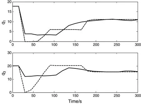
The optimal adjusting control of set point of level=9 and pH=9,with the initial state at level=14 and pH=7.The optimization problem is constructed in latent space and the Matlab optimization toolbox is used to solve the problem.The constraints are represented using original variable expressions(constraint 1)and Hotelling T2statistics(constraint 2),and the optimal trajectories are shown in Figs.8 and 9.Withoriginalphysicalvariable constraint,the optimalvalue ofobjective function is 53.3127 and the elapsed time is 8.079 s,while with the T2statistics value based constraint,they are 76.2125 and 4.805 s,respectively.Although the objective function value is larger with T2statistics constraint,its computing time cost is less.The results show that the time for controlled variables with statistics constraint to increase to set points is slightly longer than that with original variable constraint,but the variances ofmanipulated variables are more stable.Thus T2statistics constraint can be used in latent variable optimization.

Table 2 Parameters for inner model

Fig.7.Modeling result for the pH neutralization process.Dashed line:model;solid line:actual values.

Fig.8.Optimal pro files for input variables.Dotted line:constraint 1;solid line:constraint 2.

Fig.9.Optimalpro files for outputvariables.Dotted line:constraint 1;solid line:constraint2.

4.2.Case 2:Polypropylene grade transition

In complex industrial process such as polypropylene grade transition process[26,27],it is dif ficult to develop exact process model.Data-based latent modeling method is often used and the proposed optimization approach can be applied.The Spheripoltechnology is used in polypropylene production process(Fig.10),consisting ofthree reactors,two liquid-phase tubular loop reactors for homopolymerization and one gas-phase fluidized bed reactor for copolymerization.The catalyst,propylene,and hydrogen are fed to the first reactor.A portion of the slurry together with pure propylene is injected to the second reactor.The product of homopolymerization is delivered to the third reactor and mixed with ethylene to produce copolymers.Various grades of polypropylene resin can be produced in this process.Melt index(MI)is an important quality variable to specify the grade of polypropylene products[28].Its value is de fined as the amount of melted polymer squeezed through a standard ori fice in 10 min.Melt index is often measured by laboratory analysis.

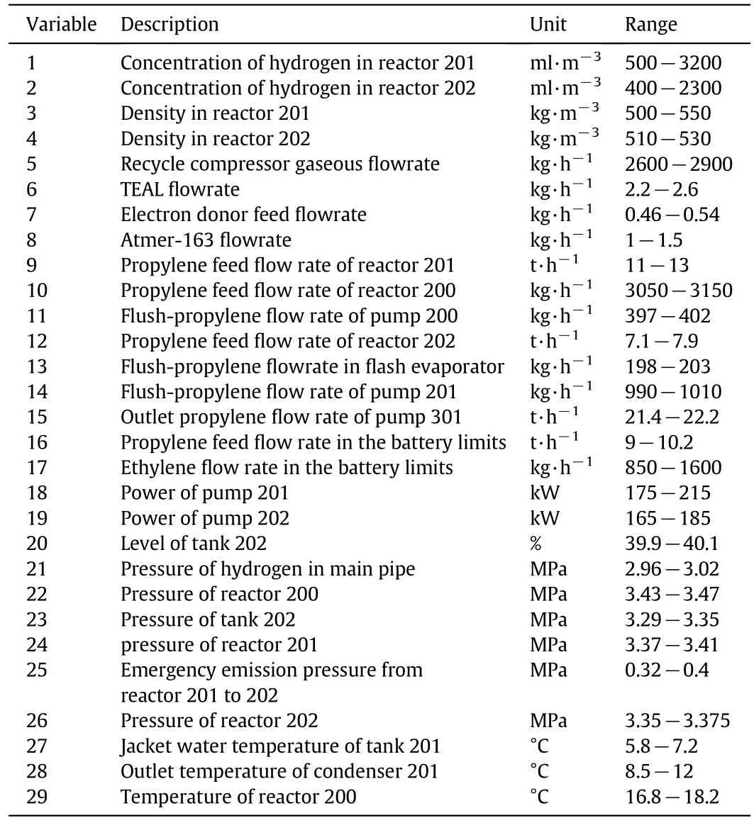
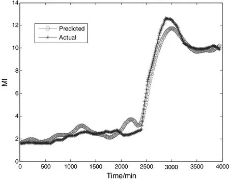
To optimize a polypropylene grade transition process,29 process variables(Table 3)are selected as the input of the PLS latent variable model.The data of polypropylene production process are collected every minute and those for training the model are resampled every 10 min.A data set with 400 sample points is used for model training,and the result is illustrated in Fig.11.The Hammerstein model order is 3 and the number of latentvariable is 5,determined by cross validation.

The optimal trajectory of quality index is shown in Fig.12.The profiles for control variables can be obtained by solving the optimization problem.In the grade transition operation of polypropylene productionprocess,optimal trajectories are determined by latent variable based dynamic optimization approach,with the constraints manipulated by Hotelling T2statistics.The optimalpro files forstate variables ofpolypropylene transition process(denoting variables in Table 3 as u1,u2,…,u29 in sequence)are shown in Figs.13 and 14.

Table 3 Process variables

Fig.11.Modeling result with Hammerstein inner relation.

Fig.10.Diagram of polypropylene production process.

Fig.12.Optimal pro file for the transition process.

5.Conclusions

In order to optimize complex operation process,a novel latent variable process optimization approach based on process data is developed.Latent variable models are used to represent the process and the Hotelling T2statistics are used to express variable constraints.Using this dynamic optimization approach,the decision variables are decreased and the computing burden is reduced.The main advantages of this optimization are that the optimization variable dimension is much less especially for complex processes and constraints can be simpli fied by Hotelling T2statistics approximation.The effectiveness of the approach with T2statistics constraint is illustrated with pH-level optimal control for neutralization process.The novel approach is also applied in practical polypropylene grade transition process and the results demonstrate the effectiveness of the methodology.Although the latent optimization approach is a practical methodology for process optimization,the feasible domain of the optimization is restricted by constraint approximation using T2statistics and the global optimum may not be guaranteed all the time.

Fig.13.Optimal pro files for state variables u1-u15.

Fig.14.Optimal pro files for state variables u16～u29.