Asymptotic Properties in a Stochastic SIRS Epidemic Model with Jumps∗

GE Qing，TENG Zhi-Dong，Xamxinur Abdurahman

(College of Mathematics and System Sciences,Xinjiang University,Urumqi Xinjiang 830046,China)

0 Introduction

As we well known,mathematical models in epidemiology have become a more and more useful tool in the analysis of spread and control of infectious diseases in host populations.The classical SIRS type epidemic dynamical model with bilinear incidence has the following form

where the homogeneous host population is subdivided into three epidemiologically distinct types of individuals,the susceptibleS,the infectiveIand the removedR.In model(1)Λ is the recruitment rate of the population;β is transmission coefficient between compartmentsSandI;µ is the natural death rate ofS,I,R;ε is the death rate due to disease;γ is the natural recovery rate of the infected individuals;δ is the rate of immunity loss ofR.

In fact,our real life is full of randomness and stochasticity.Therefore,using stochastic models can gain more real bene fits.In recent years,stochastic epidemic models with white noise perturbations have been studied by many authors[2–5].However,in the real life there are other kinds of stochastic perturbations,except to the white noise.The population may suffer sudden environmental shocks,earthquakes,etc.Now the models with only white noise cannot explain such phenomena.In order to explain these phenomena,some scholars introduce a jump process into the underlying population which is more feasible and realistic[6–10].In[9],the authors investigated the dynamics of competitive Lotka-Volterra systems with jumps and in[10],the authors investigated the asymptotic behavior of a stochastic SIR model with jumps.

Motivated by the above results,in this paper we consider a class of SIRS epidemic model with white noise and jumps as follows

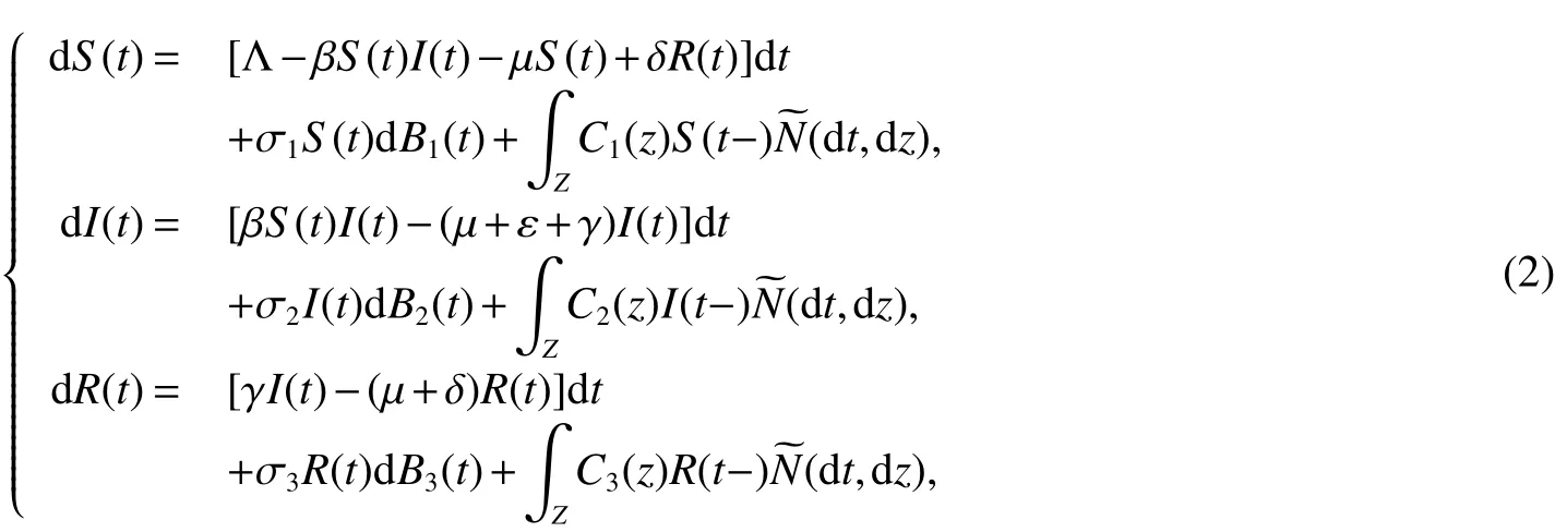
whereBi(t)(i=1,2,3)is a standard Brownian motion de fined on a complete probability space(Ω,F,P)with the filtration{F}t≥0satisfying the usual condition.≥ 0 represents the intensities ofBi(t).S(t−),I(t−)andR(t−)denote the left limit ofS(t),I(t)andR(t)at timet,respectively.(t,Z)is the compensated Poisson random measure and(t,Z)=N(t,Z)−tπ(Z),whereN(t,Z)is a Poisson random measure which is often used to describe jumps of stochastic process and is de fined on measurable subsetZof[0,∞).Characteristic measure ofN(t,Z)is denoted by π with π(Z)<∞.We assumeCi(z)>−1(i=1,2,3).We can see that ifCi=0,model(2)becomes to the following stochastic model with only white noise

For model(2),the main focus of this paper is to study how environment fl uctuations affect disease dynamics through investing the global dynamics of SIRS model with jumps.The organization of this paper is as follows.In Section 2,we show that model(2)has a unique positive solution of model(2)for any positive initial value.In Section 3 and Section 4,we show how the solution spirals around the disease-free equilibrium and endemic equilibrium of deterministic system under some conditions.

1 Global positive solution

Throughout this paper,={(S,I,R):S>0,I>0,R>0},and for the jump diffusion coefficient we assume that

(A1)For each constantm>0 there existsLm>0 such that when|x|∨|y|≤m,

whereH1(x,z)=C1(z)S(t−),H2(x,z)=C2(z)I(t−)andH3(x,z)=C3(z)R(t−).

(A2)There exists a positive constantMsuch that

SinceS(t),I(t)andR(t)in model(2)are the sizes of the susceptible,infected and recovered at timet,respectively,they should be nonnegative.Therefore,we are only interested in positive solutions.In order to get a unique global solution(i.e.,no explosion in a finite time)for any given initial value,in this section,using the Lyapunov function method,we shall show the jump processes can suppress the explosion and the solution of model(2)is positive and global as well as just containing Brownian motion.

Theorem 1Assume that(A1)and(A2)hold.Then for any initial value(S(0),I(0),R(0))∈model(2)has a unique solution(S(t),I(t),R(t))de fined for allt≥0 and the solution remains inwith probability one.

ProofWith condition(A1)as well as the drift and the diffusion are locally Lipschitz,for any initial value(S(0),I(0),R(0))∈there is a unique local solution(S(t),I(t),R(t))de fined ont∈[0,τe)satisfyingfor allt∈ [0,τe)almost surely,where τeis the explosion time.If we can show that τe= ∞a.s.,then it will be completed the proof.

Letk0be a large enough integer such thatS(0),I(0)andR(0)lie within the interval[,k0].For any intervalk≥k0,de fine the stopping time as follows

Here,throughout this paper we set inf∅ = ∞ (∅ denotes the empty set).It is clear that τkis increasing askincreases.Since τk≤ τe,we can set τ∞=limk→∞τkand τ∞≤ τe.Obviously,if we can show τ∞= ∞a.s.,then τe= ∞a.s.Suppose that the statement is false,then there exist a pair of constantsT>0 and 0<ε<1 such that

Thus,there is an integerk1≥k0such that

Now,we de fine aC2− functionF:R3+→R+as follows:

The nonnegativity of this function can be seen fromapplying It’s formula,we have

where

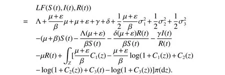
Then from(A2)and inequalityx−log(x+1)≥0 for allx>−1,we have

where

Therefore,

Integrate both sides of(5)from 0 to τk∧Tand take the expectations,we have

Let Ωk={τk≤T}fork≥k1.By(4)we haveP(Ωk)≥ ε.From the de finition of the stopping time,we can learn that for every ω ∈ Ωkthere isS(τk,ω)orI(τk,ω)orR(τk,ω)no less than eitherkor no more than.Hence by(6)yields

whereIΩkis the indicator function of Ωk.Lettingk→∞ in above inequality which leads to the contradiction.

then we have τ∞=∞a.s..Therefore,τe=∞.This completes the proof.

2 Asymptoticbehaviorarounddisease-freeequilibriumofdeterministicmodel

Model(1)always has disease-free equilibriumE0(,0,0).IfR0≤1,thenE0is globally asymptotically stable.But model(2)has no the disease-free equilibrium.Therefore,we will study the asymptotic behavior aroundE0of solution of model(2).Let

Theorem 2Assume thatR0≤1 andk1>0,k2>0,k3>0.Then for any initial valuesolution(S(t),I(t),R(t))of model(2)has the property

wherek=min{k1,k2,k3}.

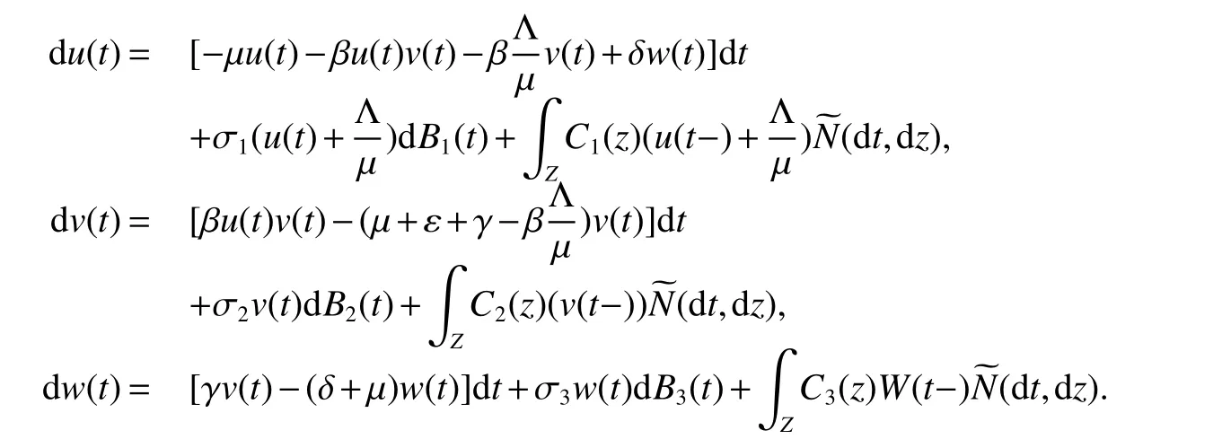
ProofLet,we can obtain thatu∈R,v>0,w>0.Then we can rewrite model(2)as follows

De fine aC2−function

Using It’s formula,we have

where

Integrating both sides of(7)from 0 tot,then taking expectation,we yields

By(8)we also have

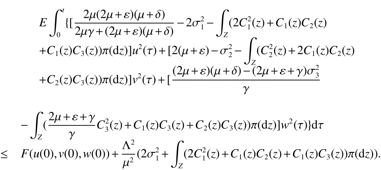
From this,we finally obtain the result of Theorem(2).This completes the proof.

Remark 1With Theorem(2),we obtain that the solution will oscillate around the disease-free equilibrium and the intensity is not only related to the value of σibutCi(z)(i=1,2,3).Further we see that the weaker the values are,the smaller the fl uctuation is,that is the smaller the stochastic perturbations,the closer to the disease-free equilibrium of model(1)the solution of model(2).

In model(2),ifCi=0(i=1,2,3)then model(2)degenerates into model(3)andk1,k2,k3of Theorem 2 become into

Then we have the following result with Theorem 2.

Corollary 1AssumeR0≤1,k11>0,k21>0 andk31>0.Then for any initial value(S(0),I(0),R(0))∈R3+solution(S(t),I(t),R(t))of model(3)has the property

wherek=min{k11,k21,k31}.

In model(2)when σi=0,Ci=0(i=1,2,3),then model(2)becomes into deterministic model(1).From(8)in Theorem 2 we obtain

Therefore,as a consequence of Theorem 2 we have the following result.

Corollary 2IfR0≤1,then disease-free equilibriumE0of model(1)is global asymptotically stable.

For model(2),if σ1=0 andC1=0,we see that model(2)has disease-free equilibriumFrom(8)in Theorem 2 we have

Therefore,as another consequence of Theorem 2 we have the following result.

Corollary 3In model(2),ifR0≤1,σ1=0 andC1=0,then there is disease-free equilibriumE0which is globally stochastically asymptotically stable.

3 Asymptotic behavior around endemic equilibrium of deterministic model

AssumeR0>1,then model(1)has endemic equilibriumE∗.But model(2)has no endemic equilibrium.On the asymptotic behavior aroundE∗of solutions of model(2)we have following result.Let

Theorem 3Assume thatR0>1,and>0,>0 and>0.Then for any initial valuesolution(S(t),I(t),R(t))of model(2)has the property

where

and

ProofDe fine aC2-functionF:R3→R+as follows,

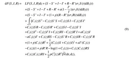
where

Using basic inequalityfor any positive constant ρ,we further have,

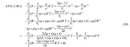
whereandMare given in the above.Integrating both sides of(9)from 0 tot,then taking expectations,it yields

Considering inequality(10)and lettingt→∞,we further obtain

This completes the proof.

Let

then as a consequence of Theorem 3 we have

Corollary 4Assume.Then for any initial value(S(0),I(0),R(0))∈solution(S(t),I(t),R(t))of model(3)has the property

where

and

References：

[1]Mena-lorca J,Hethcote H W,Dynamic models of infectious diseases as regulations of population sizes[J].Math Biol,1992,30:693-716.

[2]Beretta E,Kolmanovskii V,Shaikhet L,Stability of epidemic model with time delays in fl uenced by stochastic perturbations[J].Math Comp Simul,1998,45:269-277.

[3]Gray A,Greenhalgh D,Hu L,Mao X,Pan J,A stochastic differential equation SIS epidemic[J].SIAM J Appl Math,2011,71:876-902.

[4]Yang Q,Jiang D,Shi N,Ji C,The ergodicity and extinction of stochastically perturbed SIR and SEIR epidemic models with staturated incidence[J].Math Anal Appl,2012,388:248-271.

[5]Mao X,Stochastic Differential Equations and Applications.Horwood,Chichester,1997.

[6]Mao X,Marion G,Renshaw E,Environmental noise suppresses explosion in population dynamics[J].Stoch Proc Appl,2002,97:95-110.

[7]Bao J,Yuan C,Stochastic population dynamics driven by L´evy noise[J].Math Anal Appl,2012,391:363-375.

[8]Bao J,Mao X,Competitive Lotka-Volterra population dynamics with jumps[J].Nonlinear Anal,2011,74:6601-6616.

[9]Zhang X,Wang K,Stochastic SIR model with jumps[J].Appl Math Letter,2013,26:867-874.

[10]Zhou X,Wang K,Numerical simulations and modeling for stochastic biological systems with jumps[J].Comm Nonl Sci Numer Simul,2014,19:1557-1568.