Projections of the Advance in the Startof the Grow ing Season during the 21st Century Based on CM IP5 Simulations

XIA JiangjiangYAN ZhongweiJIA GensuoZENG Heqing Philip Douglas JONESZHOU Wenand ZHANG Anzhi

1Key Laboratory of Regional Climate-Environment for East Asia,Institute of Atmospheric Physics, Chinese Academy of Sciences,Beijing100029

2Ministry of Environmental Protection of Jiuzhaigou Country,Sichuan623400

3Climatic Research Unit,University of East Anglia,Norwich,UK

4Center of Excellence for Climate Change Research and Department of Meteorology, King Abdulaziz University,Jeddah,Saudi Arabia

5Guy Carpenter Asia-Pacific Climate Impact Centre,School of Energy and Environment, City University of Hong Kong,Hong Kong

Projections of the Advance in the Startof the Grow ing Season during the 21st Century Based on CM IP5 Simulations

XIA Jiangjiang∗1,YAN Zhongwei1,JIA Gensuo1,ZENG Heqing2, Philip Douglas JONES3,4,ZHOU Wen5,and ZHANG Anzhi1

1Key Laboratory of Regional Climate-Environment for East Asia,Institute of Atmospheric Physics, Chinese Academy of Sciences,Beijing100029

2Ministry of Environmental Protection of Jiuzhaigou Country,Sichuan623400

3Climatic Research Unit,University of East Anglia,Norwich,UK

4Center of Excellence for Climate Change Research and Department of Meteorology, King Abdulaziz University,Jeddah,Saudi Arabia

5Guy Carpenter Asia-Pacific Climate Impact Centre,School of Energy and Environment, City University of Hong Kong,Hong Kong

It is well-known that global warm ing due to anthropogenic atmospheric greenhouse effects advanced the start of the vegetation grow ing season(SOS)across the globe during the 20th century.Projections of further changes in the SOS for the 21stcentury under certain em issions scenarios(Representative Concentration Pathways,RCPs)are useful for improving understanding of the consequences of globalwarm ing.In this study,we fi rstevaluate a linear relationship between the SOS (defined using the normalized difference vegetation index)and the April temperature for most land areas of the Northern Hem isphere for 1982–2008.Based on this relationship and the ensemble projection of April temperature under RCPs from the lateststate-of-the-artglobal coupled climate models,we show the possible changes in the SOS for mostof the land areas of the Northern Hem isphere during the 21st century.By around 2040–59,the SOS w illhave advanced by-4.7 days under RCP2.6,-8.4 days under RCP4.5,and-10.1 days under RCP8.5,relative to 1985–2004.By 2080–99,itw illhave advanced by-4.3 days under RCP2.6,-11.3 days under RCP4.5,and-21.6 days under RCP8.5.The geographic pattern of SOS advance is considerably dependenton thatof the temperature sensitivity of the SOS.The larger the temperature sensitivity, the larger the date-shift-rate of the SOS.

startof grow ing season(SOS),normalized difference vegetation index(NDVI),temperature sensitivity,Representative Concentration Pathways(RCPs),CM IP5

1.Introduction

Understanding how plant species have responded to global warm ing provides background information for predicting future changes in ecosystems.A number of previous studies have reported linear relationships between temperature and vegetation grow ing season indices for different regions.Regression results suggest thatan increase of 1◦C in the average of an appropriate combination of monthly temperatures leads to differentshifts of the tim ing of the grow ing season(especially for the startof the grow ing season,SOS) for various species and locations across the world(Menzel and Fabian,1999;Sparks,2000;Chen and Pan,2002;Sparks and Menzel,2002;Fitter and Fitter,2002;Matsumoto et al.,2003;Chm ielewski et al.,2004;Piao et al.,2006;Dai et al.,2013,2014;Ge et al.,2014b;Wang et al.,2014). These results were obtained using phenologicalobservations (such as fi rst-flowering data and bud-burst-date data)as well as satellite-measured normalized difference vegetation index (NDVI)data.Shen etal.(2014)defined the temperature sensitivity of SOS as the phenological change per unit temperature and demonstrated that both the magnitude of the preseason temperature increase and the temperature sensitivity of the SOS can infl uence the advance of the SOS,which has been shown by observations during the last few decades(Lin-derholm,2006;Jeong etal.,2011).It is implied thatan appropriate combination ofmonthly temperatures may be used as a proxy of the SOS when phenological data are notavailable for the past,or for the future.

Globalwarm ing caused an extension of the grow ing season during the 20th century(Linderholm,2006).According to IPCC(2013),globalwarm ing since 1950 isvery likely due to the observed increase in anthropogenic atmospheric greenhouse gas(GHG)concentrations,and this increase is almost certain to continue in the future.The long-lived GHG concentrations exerta strong control on the radiative forcing of the climate system,and then the ecosystem.It is beneficial to analyze possible impacts of globalwarm ing on the growing season in the future.The Coupled Model Intercomparison Project Phase 5(CM IP5)projections of climate change are forced by GHG emission scenarios consistent w ith the Representative Concentration Pathways(RCPs),which were formulated based on the projected population grow th,technological development,and societal responses in the future (Moss et al.,2010).The RCP scenarios provide a rough estimate of the fi xed radiative forcing by 2100(Taylor et al., 2012).The outputof climate models under the RCP scenarios provides a base forstudying possible changes in the SOS for the 21stcentury.

A key question is whether the temperature sensitivity of the SOS remains constant at the century scale.In Shen et al.(2014),the temperature sensitivity was determ ined using the NDVI-derived SOS and effective pre-season temperature during 1982–2008.Wang etal.(2014)argued that the temperature sensitivity of a spring phenology index may change in time over a long period.However,Xia etal.(2013)found thatifonly the Apriltemperature isused,the temperature sensitivity isrobustthroughouta century-scale period atdifferent sites for mostof the land areas of the Northern Hemisphere. In the presentstudy,we investigate changes in the SOS under the RCP scenarios using the know ledge obtained from Xia et al.(2013).

It is clear that climate models are not perfect(Reichler and Kim,2008;Knutti,2008),but there have been substantial improvements from one generation of models to another [e.g.from CM IP1 to CM IP3,as summarized by Reichler and Kim(2008),and from CM IP3 to CM IP5,as summarized by Knuttiand Sedlacek(2013)].In fact,many coupled climate models w ith all radiative forcings perform well in simulating the global and northern hem ispheric mean surface air temperature evolutions of the 20th century(Cubasch etal.,2001; Zhou and Yu,2006;Meehl et al.,2007;Hegerl et al.,2007; Randall et al.,2007;Knutti et al.,2008).The consistency among models suggests that the projected changes for largescale climate features are structurally stable(M cWilliams, 2007).

The aim of this study is to reveal possible shifts of the SOS during the 21stcentury in the land areas of the Northern Hemisphere by using the established linear relationship and CM IP5 monthly temperature simulations.The study includes the follow ing steps:

(1)Evaluate the relationship between the SOS and April temperature(temperature sensitivity of SOS)based on observational data for 1982–2008 and reconstruct the SOS time series for the same period.

(2)Evaluate the performance of CM IP5 coupled models by comparing the observed changes in monthly mean temperature and the simulated results for the past.

(3)Quantify the possible changes in SOS for 2006–99 under the RCP scenarios w ith an uncertainty assessment.

2.Data

2.1.Temperature

This study uses the global 0.5◦×0.5◦gridded land surface monthly(April)mean air temperature dataset(TS 3.10)for 1901–2008,developed at the Climatic Research Unit(CRU)(Harris et al.,2014).This dataset were obtained from the Climatic Research Unit,University of East Anglia,via their website(accessed 16 March 2014): http://badc.nerc.ac.uk/view/badc.nerc.ac.uk ATOM dataent 1256223773328276.

2.2.NDVI data

NDVIdata have been developed from the Advanced Very High-Resolution Radiometer(AVHRR)onboard the National Oceanic and Atmospheric Adm inistration’s(NOAA)polarorbiting satellites.The data are calibrated and processed by the National Aeronautics and Space Adm inistration’s (NASA)Global Inventory Monitoring and Modeling Systems (GIMMS)group,w ith a spatial resolution of8 km×8 km and a temporalresolution of15 days,for1982–2008.Furtherdata corrections(e.g.aerosol,cloud,volcanic,and sensor degradation)are also applied to improve the data quality(Tucker et al.,2005).The temperate vegetation areas of the Northern Hemisphere are chosen as the study area,where the seasonality of vegetation is evident(Slayback etal.,2003;Piao et al.,2006).The NDVI changes could be used to describe the“greenness”of vegetation.In this study,for each gird, the thresholds for the SOS are defined from the NDVI climatology.In the climatological annual cycle of NDVI,the SOS is determined by detecting the inflection date when this NDVI annual cycle time series begins to rise for a specific year(Zeng etal.,2011;Jeong etal.,2011).

2.3.CM IP5 output

The simulations of global coupled ocean–atmosphere general circulation models(CGCM s)provide the primary base for studying possible future climate changes(Kharin etal.,2007).The CM IP5 projections of climate change are forced by GHG emission scenariosconsistentwith the RCPs, as described in Moss etal.(2010).

In this study,the RCP2.6,RCP4.5 and RCP8.5 scenarios are chosen to represent a range of possible outcomes for 2006–99(Table 1).The radiative forcing under RCP8.5 increases throughout the 21st century,and reaches a level of about8.5 W m-2by 2100.In addition to this“high”RCP8.5 scenario,there is an intermediate scenario,RCP4.5,whichreaches a level of about 4.5 W m-2by 2100.The RCP2.6 scenario is described as a peak-and-decay low scenario,in which the radiative forcing reaches a maximum near the m iddle of the 21st century before decreasing to an eventual low levelof 2.6 W m-2(Taylor etal.,2012).

Table 1.Details of the RCPs.

A collection of models can be used to determine the uncertainty range in projections(Tebaldiand Knutti,2007).In this study,we select16 CM IP5 models developed by 12 scientific organizations from 8 countries around the world(Table 2).The average of multiple models(multi-modelensemble,MME)performsbetter than any single modelwhen compared w ith observations(Gillettetal.,2002;Gleckler etal., 2008;Reichler and Kim,2008).In this study,we calculate the MME by averaging the results of the 16 models.Details of all the experiments and output of the models used in this study were obtained from the Working Group on Coupled Modelling(WGCM)under the World Climate Research Programme(WCRP),via their website(accessed 1 September 2013):http://cm ip-pcmdi.llnl.gov/cm ip5.

3.M ethod

To evaluate the performance of the CGCM s from CM IP5 in reproducing the current climate,simulations of the 20th century experiments,termed“historical”,are compared w ith the observations,for 1901–2004.The historical runs are driven by observed atmospheric composition changes(including both anthropogenic and natural sources).The historical scenarios cross much of the industrial period(from the 19th century to the present).Based on these results,the projection of monthly mean temperature change(then the changes in grow ing season indices)over the globe in the 21st century is discussed.

For convenience of comparison w ith high-resolution NDVI data,we assume that large-scale climate change in temperature is in general of good spatial homogeneity,and hence the CRU observational data and the CGCM s’output are interpolated into a common grid of 8 km×8 km.This may lose some NDVI information at the finer-scale grids, but hopefully this does not have much effect on the results at the large-scale(hemispheric scale)for the pattern of SOS changes.

For each grid,the linear regression coefficient between shifts of the SOS and changes in corresponding Aprilmean temperature is quantified for1982–2008,using least-squares methods.The coefficient is defined as the temperature sensitivity of the SOS for each grid.Only grids show ing significant correlation(w ith a significance level of 0.05)are considered in this study.Figure 1a shows an example of the temperature sensitivity of the SOS averaged over the analyzed areas(all the grids show ing significant correlation).It indicates that for a 1◦C warm ing of the Aprilmean temperature, there should be an advancementof 2.1 days for the SOS.

This linear relationship,i.e.the temperature sensitivity of the SOS,enables us to straightforwardly reconstruct the SOS time series.First,the April temperature anomalies are calcu-lated w ith respectto the whole period foreach grid.Then,the April temperature anomalies multiplied by the temperature sensitivity of the SOS defines the reconstructed SOS series for a given grid.

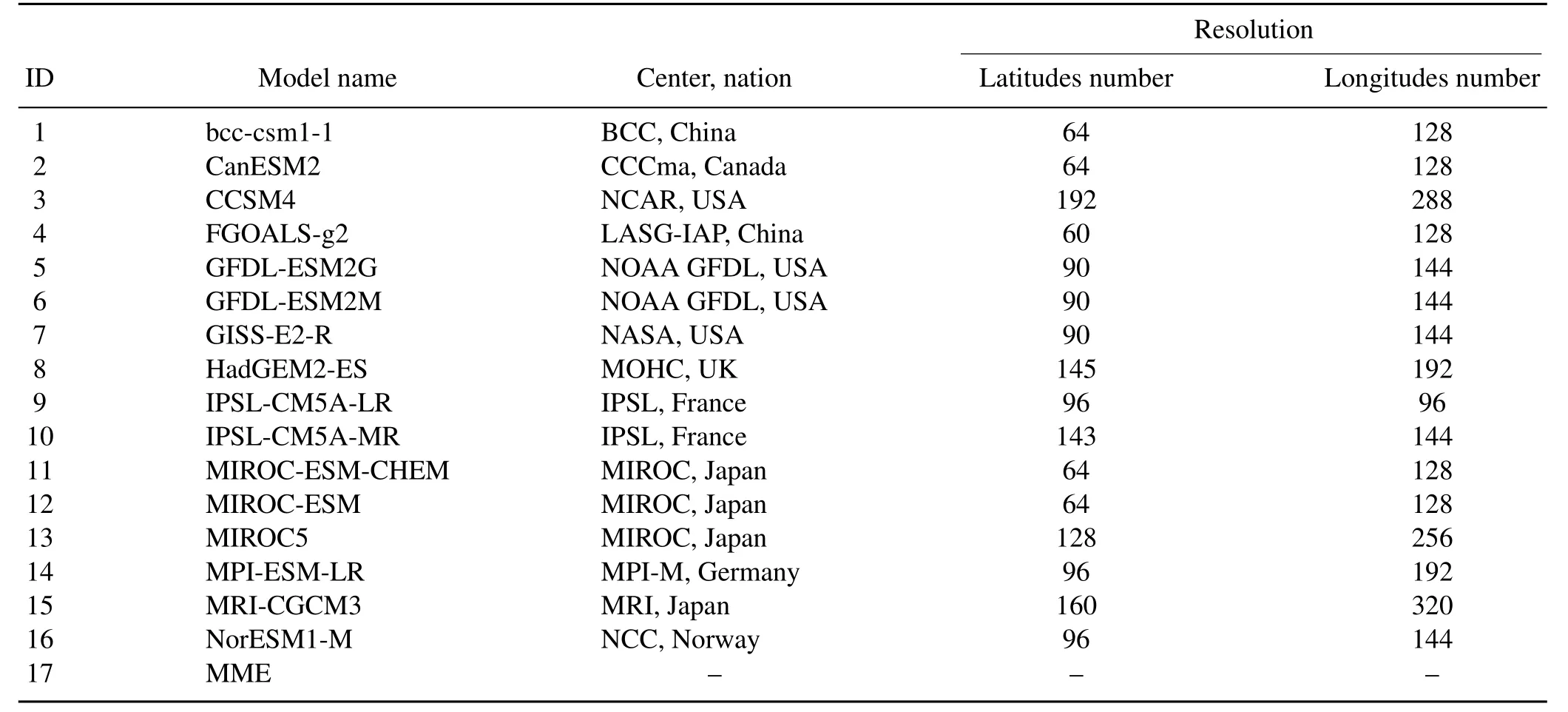
Table 2.Details of the CM IP5 models used in this study.

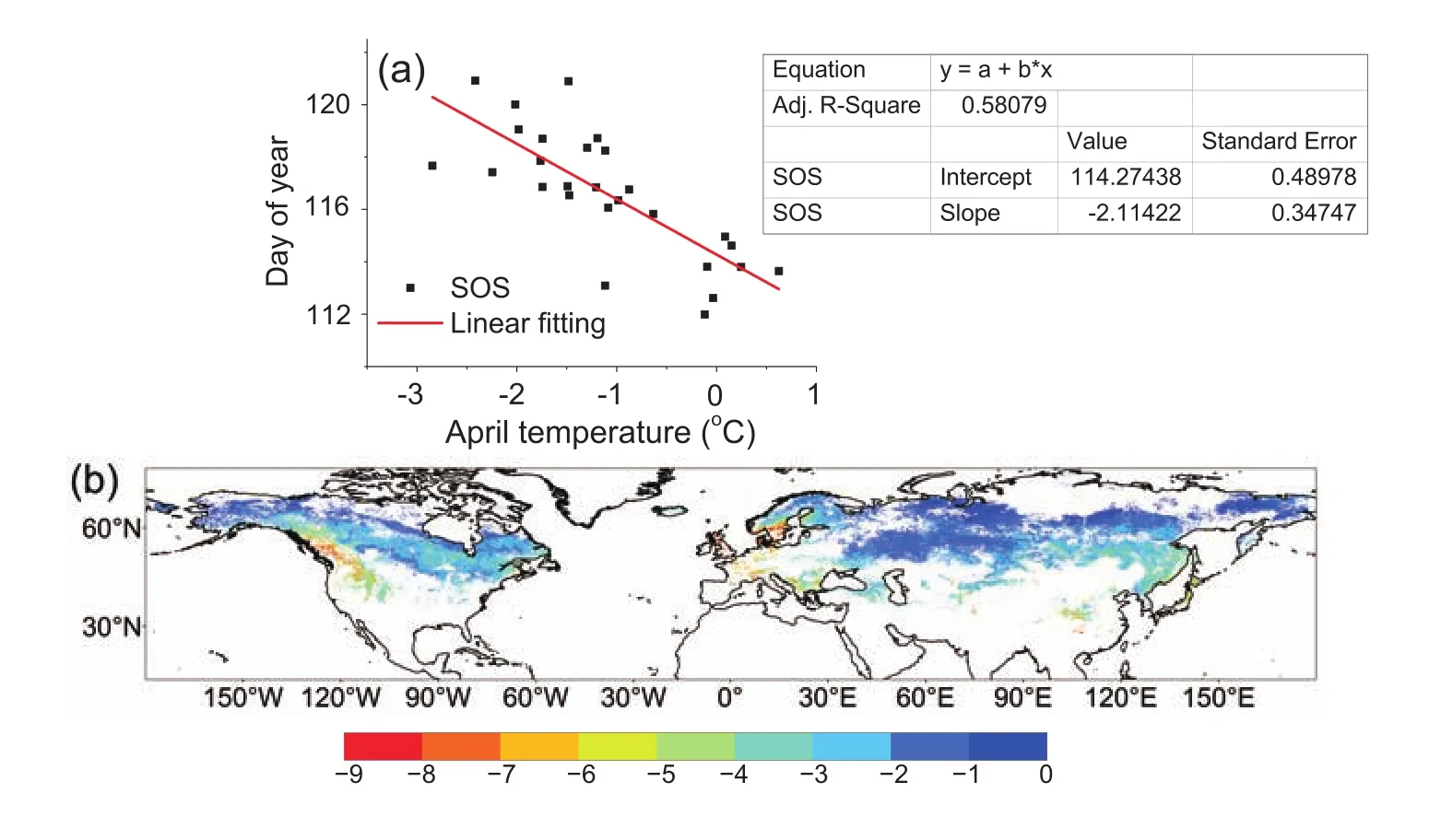
Fig.1.Temperature sensitivity of the SOS,e.g.the regression coefficients of the SOS onto April temperature for 1982–2008,(a)averaged over the analyzed areas and(b)at each grid. Only grids that show a significant linear relationship are marked(significance level:0.05). Units:d◦C-1.

4.Results

4.1.Temperature sensitivity of the SOS

The regression coefficients of the SOS on the April temperature range from-0.8 to-5 d◦C-1(5%to 95%)formost of the land areasof the Northern Hemisphere(Fig.1b,mainly located between 30◦N and 70◦N).These linear regression coefficients are considered to represent the temperature sensitivity of SOS.The spatial distributions of the phenological sensitivity span a latitudinalgradientover the continents and a longitudinal gradient in the coastal zones,show ing larger values in southwestern North America,western Europe,and southern Asia.This pattern is consistent w ith the previous study of Xia etal.(2013).

In response to climate warming,shifts of the SOS in the temperate zones are determined notonly by the temperature level in time but also by the temperature sensitivity.Having considered both factors,we reconstruct the time series of the SOS(the expected SOS).From 1982 to 2008,mostof the analyzed areas experience advanced SOS,forboth the observed (Fig.2a)and expected(Fig.2b)SOS.This is consistentw ith the previous study of Jeong etal.(2011).The geographical distribution of the trends derived from the expected SOS(Fig. 2b)is broadly consistentspatially w ith those of the observed trends,though in general the expected trends are smaller in magnitude than the observed.

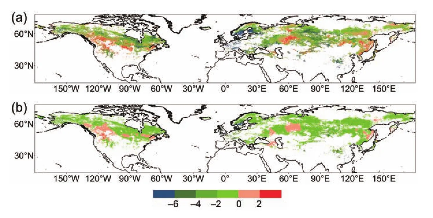
Fig.2.(a)Spatial distribution of the linear trends of the observed SOS.(b)The same as(a), except for the expected(reconstructed)SOS.Units:d(10 yr)-1.

On average over the analyzed areas,the trends of the observed SOS(Fig.3)are-1.5 d(10 yr)-1,while those for the expected SOS are-0.8 d(10 yr)-1.The trends of the reconstructed indices explain only abouthalf of the observed trends.This is partly because the SOS is notdeterm ined only by temperature,but also other factors such as precipitation and humidity,which may change and/or reinforce the effect on phenology induced by climatic warm ing.Nevertheless, even based on the same AVHRR dataset,there is large uncertainty in estimating the phenological trends[e.g.they range from 0.4 to 1.9 d(10 yr)-1for China(Cong et al.,2013)], depending on the different methods applied to quantify the phenologicaldates.In comparison,the rate ofadvance of the expected and observed SOS are very sim ilar from the early 1990s.The correlation coefficients are about0.8 between the observed and expected time series for1982–2008.It is clear that the reconstructed phenological indices can capture the main features as observed on a hem ispheric-scale analysis.

Itcan be concluded that this linear relationship enables us to study phenological changes in the SOS by using monthly mean temperature when NDVIdata are notavailable,e.g.the changes in SOS under the RCP scenarios in the 21stcentury.

4.2.Projection of changes in the SOS under RCPs

Many coupled climate models have the ability to simulate both the globaland Northern Hemisphere mean surface air temperature evolutions of the 20th century(Zhou and Yu, 2006;Hegerletal.,2007;Randalletal.,2007;Knutti,2008; IPCC,2013).It is clear that the performances of the CGCMs in reproducing the historicalchangesin April temperature are good enough that they can be used for projecting changes in the SOS in the future w ith reasonable confidence.In this study,we simply evaluate the behavior of the CGCM s from CM IP5 based on the April temperature,averaged over the Northern Hem isphere.

Fig.3.Interannual variations in the observed(blue)and expected(red)SOS.Correlation between the two time series is given in the lower-rightcornerof the figure.

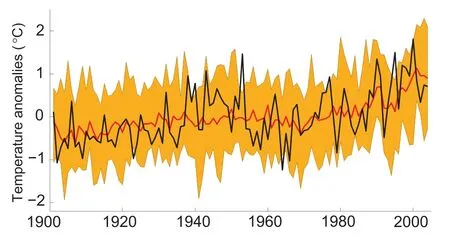
Fig.4.Comparison of the observed(black line)northern hem ispheric–scale changes in surface temperature anomalies (relative to the average for the whole period)of Aprilw ith results simulated(red line)by climate models under the historical scenario for 1901–2004.Yellow shaded bands show the 5%to 95%uncertainty range for these simulations from the 16 climate models.

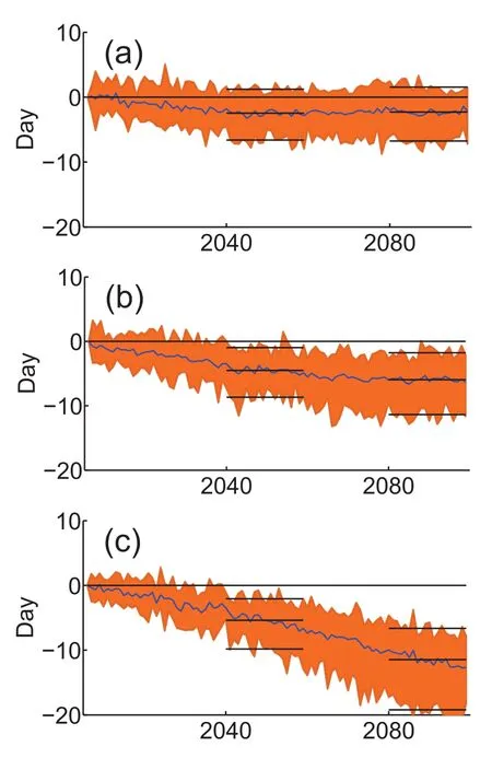
Fig.5.The SOS time series averaged over the Northern Hemisphere during 2006–99 w ith respect to 1985–2004(historical scenario),projected by the CM IP5 models under the(a) RCP2.6,(b)RCP4.5,and(c)RCP8.5 scenarios.Negative(positive)values indicate the advance(delay)in the number of days w ith respect to 1985–2004.Orange shaded bands show the 5% to 95%uncertainty range for these simulations from the 16 climate models.The short horizontal lines indicate the averaged SOS for 2040–59 and 2080–99,w ith the m iddle ones being the SOS calculated from the MME,and the upper and lower ones the 5%and 95%ranges,respectively.

Figure 4 shows that the observed April temperature,averaged over the Northern Hem isphere,shows an increasing trend for the whole period studied,w ith a rate of about 0.11◦C(10 yr)-1.It also shows a multi-decadal variance,which experiences two increasing periods(from 1901 to the m id-1940s and from the mid-1960s to 2004).Between these increasing periods there is a decreasing period.The MME April temperature shows sim ilar variance to the observed one,including the increasing trend for the whole period[0.09◦C(10 yr)-1].The 5%–95%uncertainty intervals assessed using the output of the 16 climate models,which are also given in Fig.4,indicate uncertainty intervals of the increasing trends from 0.04◦C to 0.14◦C(10 yr)-1for the simulated April temperature for the whole period.The increasing trends of April temperature between the observations and the simulations for 1951–2004 are also compared.The trend is 0.21◦C(10 yr)-1for the observations,while the trend is 0.19◦C(10 yr)-1for the MME[w ith uncertainty intervals of 0.09◦C to 0.27◦C(10 yr)-1].This indicates that the CGCM s have the ability to simulate the April temperature changes on a hemispheric scale fordifferentperiods.

The simulated SOS shows sustained advancing trends for 2006–99 under the RCP4.5(Fig.5b)and RCP8.5(Fig.5c) scenarios.For the RCP2.6 scenario(Fig.5a),the SOS sustains an advancement rate for 2006–40,while from 2040 onwards the SOS is almost the same.The SOS calculated from the MME advances(negative value)-2.5 days(uncertainty intervalcalculated from the 16 simulations:-6.6 to 1.2 days)under RCP2.6,-4.5 days(-8.7 to-1.0 days)under RCP4.5,and-5.4 days(-9.8 to-2.0 days)under RCP8.5, when comparing 2040–59 w ith 1985–2004.The SOS advances-2.3 days(-6.8 to 1.5 days)under RCP2.6,-6.0 days(-11.0 to-1.8 days)under RCP4.5,and-11.5 days (-19.2 to-6.6 days)underRCP8.5,when comparing 2080–99 w ith 1985–2004.This indicates that the future projections of changes show a high degree ofuncertainty,butconsistency in the advancementdirection.

Figures 6 and 7 show the changes in the SOS under the RCP scenarios for 2040–59 and 2080–99,respectively,in terms of the results of the historical scenario for1985–2004. The patterns are sim ilar among these six geographicalmaps of changes in the SOS.The patterns of changes in the SOS under the RCP scenarios are different from the observed for the last few decades in some aspects.For example,greater advancement trends are observed in Europe(Fig.2a);while in the CM IP5 simulations,the larger changes in the SOS during the 21st century are in southwestern North America, western Europe,southern Asia,and parts of eastern Canada. It is worth noting that this pattern is sim ilar to the pattern of temperature sensitivity of the SOS(Fig.1),indicating that the regions w ith larger SOS temperature sensitivity need to have more attention paid to them.

In addition,by comparing the land cover categories for 2006 using NASA’s Moderate Resolution Imaging Spectroradiometer(MODIS)(MCD12C1,collection V051,were obtained from the Land Processes Distributed Active Archive Center,via their website:https://lpdaac.usgs.gov/products/ modis productstable/m cd12c1,accessed 10 August 2013), we found that the areas w ith large changes in SOS are mainly covered by evergreen needleleaf forest,m ixed forest,and grasslands.For these regions,the simulated changes in the SOS imply considerable influences on the ecosystem structure and function,which deserve further study.

5.Discussion

Fig.6.Changes in the SOS for(a)RCP2.6,(b)RCP4.5 and(c)RCP8.5 for 2040–59 w ith respect to the results of 1985–2004 under the historicalscenario,calculated from MME.Units:d.

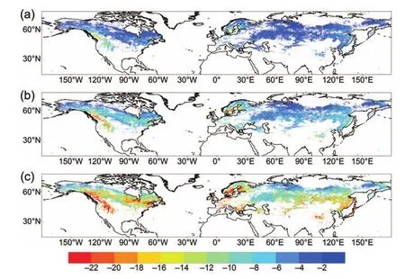
Fig.7.Changes in SOS for(a)RCP2.6,(b)RCP4.5 and(c)RCP8.5 for 2080–99 w ith respect to the results of1985–2004 under the historicalscenario,calculated from MME.Units:d.

This study investigated the possible changes in the SOS forparts of the land areas of the Northern Hemisphere during the 21st century,based on the temperature sensitivity of the SOS and the April temperature projected under the RCP scenarios from the lateststate-of-the-art CGCMs.Itwas found that the observed trend of the SOS is-1.5 d(10 yr)-1but the simulated one is-0.8 d(10 yr)-1for 1982–2008(Fig. 3),implying that the models underestimate the trend of the SOS by a factorof 1.875.We suggest that the projected SOS trends under the three RCPs scenarios should be multiplied by 1.875.Therefore,the SOS based on the MME simulation w illadvance by-4.7 days under RCP2.6,-8.4 days under RCP4.5,and-10.1 daysunderRCP8.5,for2040–59 relative to 1985–2004.Itw illadvance by-4.3 days under RCP2.6, -11.3 days under RCP4.5,and-21.6 days under RCP8.5 for2080–99 relative to 1985–2004.Itis worth noting that the advance of the SOS during the 21st century shows large regionaldifferences.Forexample,averaged over the study areas in China(20◦–42◦N,95◦–120◦E),the SOS w illadvance (the values in Fig.7 multiplied by 1.875)by-10.7 days under RCP2.6,-18.6 days under RCP4.5,and-37.5 days under RCP8.5 for 2080–99 relative to 1985–2004.These are larger than the results obtained by Ge et al.(2014a),who suggested that,in China during the 21stcentury,the average numberofdays by which the fi rst leaf date advances is about -19 days,-11 days and-7.4 days under the IPCC(2001) A2,A1B and B2 scenarios,respectively.This discrepancy is partly due to the differences of temperature changes between the RCP scenarios and the previous versions of the scenarios.Comparing the temperature sensitivity of the SOS(Fig. 1)and the changes in the SOS for the 21st century(Figs.6 and 7),we can conclude that the larger the local temperature sensitivity of the SOS,the more notable the shiftof the SOS, i.e.in southwestern North America,western Europe,southern Asia,and parts ofeastern Canada.

Acknow ledgements.This work was supported by the CAS Strategic Priority Research Program—Climate Change:Carbon Budget and Relevant Issues(Grant No.XDA05090000),CityU Strategic Research(Grant No.7004164),and the National Natural Science Foundation of China(ProjectNo.41405082).

REFERENCES

Chen,X.Q.,and W.F.Pan,2002:Relationships among phenological grow ing season,time-integrated normalized difference vegetation index and climate forcing in the temperate region of eastern China.Int.J.Climatol.,22,1781–2002.

Chm ielewski,F.M.,A.Muller,and E.Bruns,2004:Climate changes and trends in phenology of fruit trees and field crops in Germany,1961–2000.Agric.Forest Meteor.,121,69–78.

Cong,N.,T.Wang,H.J.Nan,Y.C.Ma,X.H.Wang,R.B.M yneni,and S.L.Piao,2013:Changes in satellite-derived spring vegetation green-up date and its linkage to climate in China from 1982 to 2010:A multimethod analysis.Global Change Biol.,19,881–891.

Cubasch,U.,and Coauthors,2001:Projections of future climate change.Climate Change 2001:The Scientific Basis.Contribution of Working Group I to the Third Assessment Report of the Intergovernmental Panel on Climate Change,J. T.Houghton et al.,Eds.,Cambridge University Press,Cambridge,UK.,525–582.

Dai,J.H.,H.J.Wang,and Q.S.Ge,2013:Multiple phenological responses to climate change among 42 plantspecies in Xi’an, China.Int.J.Biometeor.,57,749–758.

Dai,J.H.,H.J.Wang,and Q.S.Ge,2014:The spatial pattern of leaf phenology and its response to climate change in China. Int.J.Biometeor.,58,521–528.

Fitter,A.H.,and R.S.R.Fitter,2002:Rapid changes in flowering time in British plants.Science,296,1689–1691.

Ge,Q.S.,H.J.Wang,and J.H.Dai,2014a:Simulating changes in the leaf unfolding time of 20 plant species in China over the twenty-fi rstcentury.Int.J.Biometeor.,58(4),473–484.

Ge,Q.S.,H.J.Wang,T.Rutishauser,and J.H.Dai,2014b:Phenological response to climate change in China:A meta-analysis. GlobalChange Biol.,doi:10.1111/gcb.12648.

Gillett,N.P.,F.W.Zw iers,A.J.Weaver,G.C.Hegerl,M.R. A llen,and P.A.Stott,2002:Detecting anthropogenic influence w ith a multi-model ensemble.Geophys.Res.Lett.,29(20),31-1–31-4,doi:10.1029/2002GL015836.

Gleckler,P.J.,K.E.Taylor,and C.Doutriaux,2008:Performance metrics for climate models.J.Geophys.Res.,113,doi: 10.1029/2007JD008972.

Harris,I.,P.D.Jones,T.J.Osborn,and D.H.Lister,2014:Updated high-resolution grid ofmonthly climatic observations—the CRU TS3.10 Dataset.Int.J.Climatol.,34,623–642.

Hegerl,G.C.,and Coauthors,2007:Understanding and attributing climate change.Climate Change 2007:The Physical Science Basis.Contribution of Working Group I to the Fourth AssessmentReportofthe IntergovernmentalPanelon Climate Change,S.Solomon etal.,Eds.,Cambridge University Press, Cambridge,United Kingdom and New York,NY,USA,663–745.

IPCC,2001:Climate Change 2001:Impacts,Adaptation,and Vulnerability.Contribution of Working Group II to the Third Assessment Report of the Intergovernmental Panel on Climate Change,J.J.M ccarthy et al.,Eds.,Cambridge University Press,Cambridge,United Kingdom and New York,NY,USA, 1032 pp.

IPCC,2013:Climate Change 2013:The physical science basis. Contribution of Working Group I to the Fifth Assessment Reportof the Intergovernmental Panel on Climate Change,T.F. Stocker etal.,Eds.,Cambridge University Press,Cambridge, United Kingdom and New York,NY,USA,1535 pp.

Jeong,S.J.,C.H.Ho,H.J.Gim,and M.E.Brown,2011:Phenology shifts at start vs.end of grow ing season in temperature vegetation over the Northern Hemisphere for the period 1982–2008.Global Change Biology,17,2385–2399,doi: 10.1111/j.1365-2486.2011.02397.x.

Kharin,V.V.,F.W.Zw iers,X.B.Zhang,and G.C.Hegerl, 2007:Changes in temperature and precipitation extremes in the IPCC ensemble of global coupled model simulations.J. Climate,20,1419–1444.

Knutti,R.,2008:Should we believe model predictions of future climate change?Philosophical Transactions of the Royal Society A,366,4647–4664,doi:10.1098/rsta.2008.0169.

Knutti,R.,and J.Sedlacek,2013:Robustness and uncertainties in the new CM IP5 climate modelprojections.Nature Climate Change,3,369–373,doi:10.1038/nclimate1716.

Knutti,R.,and Coauthors,2008:A review of uncertainties in global temperature projections over the twenty-fi rst century. J.Climate,21,2651–2663,doi:10.1175/2007JCLI2119.1.

Linderholm,H.W.,2006:Grow ing season changes in the last century.Agric.Forest Meteor.,137,1–14,doi:10.1016/ j.agrformet.2006.03.006.

Matsumoto,K.,T.Ohta,M.Irasawa,and T.Nakamura,2003:Climate change and extension of the Ginkgo biloba L.grow ing season in Japan.Global Change Biology,9,1634–1642,doi: 10.1046/j.1529-8817.2003.00688.x.

McWilliams,J.C.,2007:Irreducible imprecision in atmospheric and oceanic simulations.Proc.Natl.Acad.Sci.USA,104, 8709–8713,doi:10.1073/pnas.0702971104.

Menzel,A.,and P.Fabian,1999:Grow ing season extended in Europe.Nature,397,659.

Meehl,G.A.,and Coauthors,2007:Global Climate Projections. Climate Change 2007:The PhysicalScience Basis.Contribution of Working Group I to the Fourth Assessment Report of the Intergovernmental Panel on Climate Change,S.Solomon et al.,Eds,Cambridge University Press,Cambridge,United Kingdom and New York,NY,USA,747–845.

Moss,R.H.,and Coauthors,2010:The nextgeneration of scenarios for climate change research and assessment.Nature,463, 747–756,doi:10.1038/nature08823.

Piao,S.L.,J.Y.Fang,L.M.Zhou,P.Ciais,and B.Zhu,2006: Variations in satellite-derived phenology in China’s temperate vegetation.Global Change Biology,12,672–685,doi: 10.1111/j.1365-2486.2006.01123.x.

Randall,D.A.,and Coauthors,2007:Climate models and their evaluation.Climate Change 2007:The Physical Science Basis.Contribution ofWorking Group I to the Fourth Assessment Report of the Intergovernmental Panel on Climate Change, S.Solomon et al.,Eds.,Cambridge University Press,Cambridge,United Kingdom and New York,NY,USA,589–662. Reichler,T.,and J.Kim,2008:How welldo coupled models simulate today’s climate?Bull.Amer.Meteor.Soc.,89,303–311, doi:10.1175/BAMS-89-3-303.

Shen,M.G.,and Coauthors,2014:Earlier-Season vegetation has greater temperature sensitivity of spring phenology in northern hem isphere.Plos One,9(2),e88178,doi:10.1371/journal.pone.0088178.

Slayback,D.A.,J.E.Pinzon,S.O.Los,and C.J.Tucker, 2003:Northern hem isphere photosynthetic trends 1982–99. Global Change Biology,9(1),1–15,doi:10.1046/j.1365-2486.2003.00507.x.

Sparks,T.,2000:The long-term phenology ofwoodland species in Britain.Long-term Studies in British Woodland,Vol.34,English Nature Science Series,K.J.Kirby and M.D.Morecroft, Eds.,98–105.

Sparks,T.H.,and A.Menzel,2002:Observed changes in seasons:An overview.Int.J.Climatol.,22,1715–1725,doi: 10.1002/joc.821.

Taylor,K.E.,R.J.Stouffer,and G.A.Meehl,2012:An overview of CM IP5 and the experiment design.Bull.Amer.Meteor. Soc.,93,485–498,doi:10.1175/BAMS-D-11-00094.1.

Tebaldi,C.,and R.Knutti,2007:The use of the multi-model ensemble in probabilistic climate projections.Philosophical Transactions of the Royal Society A,365,2053–2075,doi: 10.1098/rsta.2007.2076.

Tucker,C.J.,J.E.Pinzon,M.E.Brown,D.A.Slayback,E.W. Pak,R.Mahoney,E.F.Vermote,and N.E.Saleous,2005: An extended AVHRR 8 km NDVI data set compatible w ith MODIS and SPOT vegetation NDVI data.Int.J.Remote Sens.,26,4485–4498.

Wang,H.J.,J.H.Dai,J.Z.Zheng,and Q.S.Ge,2014:Temperature sensitivity of plant phenology in temperate and subtropical regions of China from 1850–2009.Int.J.Climatol.,doi: 10.1002/joc.4026.

Xia,J.J.,Z.W.Yan,and P.L.Wu,2013:Multidecadalvariability in localgrow ing season during 1901–2009.Climate Dyn.,41, 295–305.

Zeng,H.Q.,G.S.Jia,and H.Epstein,2011:Recent changes in phenology over the northern high latitudes detected from multi-satellite data.Environ.Res.Lett.,6(4),045508,doi: 10.1088/1748-9326/6/4/045508.

Zhou,T.J.,and R.C.Yu,2006:Twentieth century surface air temperature over china and the globe simulated by coupled climate models.J.Climate.,19(22),5843–5858.

:Xia,J.J.,Z.W.Yan,G.S.Jia,H.Q.Zeng,P.D.Jones,W.Zhou,and A.Z.Zhang,2015:Projections of the advance in the start of the grow ing season during the 21st century based on CM IP5 simulations.Adv.Atmos.Sci.,32(6),831–838,

10.1007/s00376-014-4125-0.

(Received 18 June 2014;revised 8 October2014;accepted 22 October2014)

∗Corresponding author:XIA Jiangjiang

Email:xiajj@tea.ac.cn

©Institute of Atm ospheric Physics/Chinese Academ y of Sciences,and Science Press and Springer-Verlag Berlin Heidelberg 2015