Fault Prediction Based on Dynamic Model and Grey Time Series Model in Chemical Processes*

TIAN Wende (田文德)**, HU Minggang (胡明刚)and LI Chuankun (李传坤)College of Chemical Engineering, Qingdao University of Science & Technology, Qingdao 6604, ChinaZibo Weichuang Petrochemical Design Co., Ltd, Zibo 55400, ChinaState Key Laboratory of Chemicals Safety, Qingdao Safety Engineering Institute, SINOPEC, Qingdao 6607 China

Fault Prediction Based on Dynamic Model and Grey Time Series Model in Chemical Processes*

TIAN Wende (田文德)1,**, HU Minggang (胡明刚)2and LI Chuankun (李传坤)31College of Chemical Engineering, Qingdao University of Science & Technology, Qingdao 266042, China2Zibo Weichuang Petrochemical Design Co., Ltd, Zibo 255400, China3State Key Laboratory of Chemicals Safety, Qingdao Safety Engineering Institute, SINOPEC, Qingdao 266071, China

This paper combines grey model with time series model and then dynamic model for rapid and in-depth fault prediction in chemical processes. Two combination methods are proposed. In one method, historical data is introduced into the grey time series model to predict future trend of measurement values in chemical process. These predicted measurements are then used in the dynamic model to retrieve the change of fault parameters by model based diagnosis algorithm. In another method, historical data is introduced directly into the dynamic model to retrieve historical fault parameters by model based diagnosis algorithm. These parameters are then predicted by the grey time series model. The two methods are applied to a gravity tank example. The case study demonstrates that the first method is more accurate for fault prediction.

fault prediction, dynamic model, grey model, time series model

1 INTRODUCTION

Chemical processes frequently involve flammable and explosive chemicals and operate under high temperature and pressure conditions. Its accidents not only result in huge economic losses but also threaten operator’s life. Detecting minor abnormal symptom and predicting its trend in time is a key to guarantee chemical production safety [1]. Some severe accidents can be avoided if operators take advantage of early warnings to detect and separate possible system faults. Fault diagnosis and fault prediction are two main methods for improving the safety of chemical industry. Fault diagnosis analyzes the data collected from chemical processes to determine whether a fault currently occurs in the process [2-4], while fault prediction utilizes the running state of chemical processes and some non-first principles model to forecast possible fault development in the near future [5-7]. In these different time domains, none of them can fulfill monitoring task completely.

The fault prediction models in literature can be classified as qualitative trend analysis, support vector regression, kernel regression, linear regression model, grey model, and time series model [8-14]. The grey model requires a small amount of data and can give an accurate trend prediction, but has a poor adaptability to data fluctuation [15-17]. In this paper, the grey model is combined with the time series model in series to correct its residuals and improve its adaptability to data oscillation. In addition, based on our earlier work on dynamic simulation based fault diagnosis [18, 19], we combine the dynamic model with grey time series model to form a hybrid fault prediction model. We will predict non-measurable fault parameters that are critical to reflect the running state of chemical process in the near future [20-22]. The two methods of combination are discussed and their effectiveness is demonstrated with a gravity tank example.

2 FAULT PREDICTION MODEL

2.1 Multi-variable grey model

General steps to build multi-variable grey model for prediction are as follows [21].

(1) Generate original sequence using untreated data

(2) Calculate the following sequence by summarizing the original sequence

where ngdenotes the number of variables and Ngdenotes the sampling number for each variable. abouWte can establish continuous-time state-space model

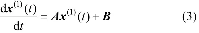
where

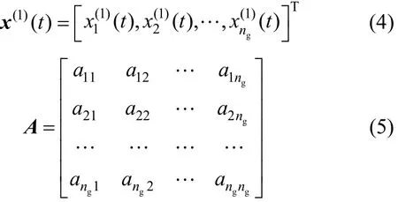
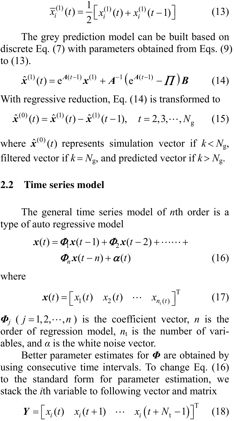
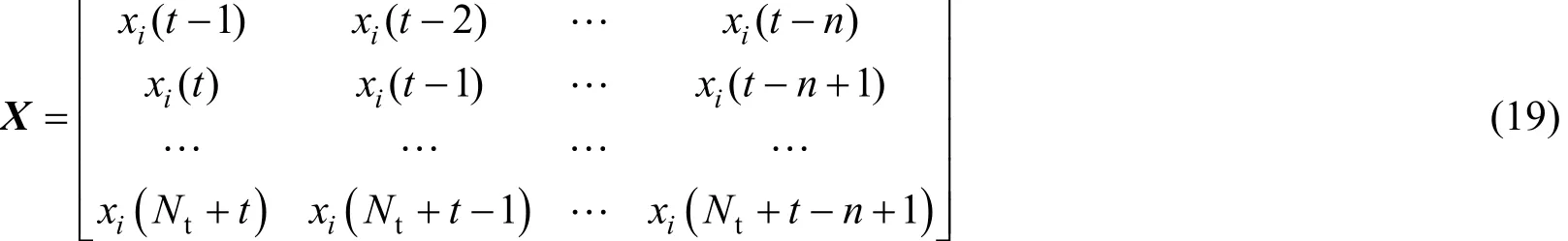
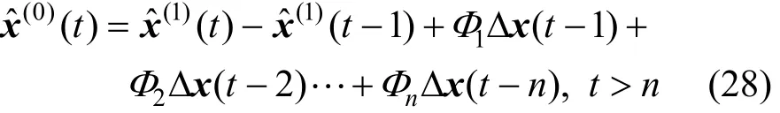
In Eqs. (23) to (25), k is the order of criterion function and Ntis the number of sampling data. The value of k that minimizes criterion function is the suitable order for Eq. (16), so that the time series model has the best prediction accuracy.

2.3 Combination of grey model with time series model and then dynamic model

Grey model accumulates untreated data [Eq. (2)] to average variations between adjacent-time data and smoothes the data slightly. It excels overall trend prediction but may introduce lagging time responding to data variation. In time series model, each data at time t is considered as a linear combination of n pieces of data before time t. Because the combination reserves variation trend between adjacent-time data as much as possible, it benefits local trend prediction greatly. The combining point between grey model and time series model lies in overall smooth trend predicted by the former plus local fluctuation trend predicted by the latter to give complete data prediction.

Grey model and time series model are good at prediction of smoothly changed data and frequently changed data, respectively. Therefore, hybrid grey time series model is proposed to utilize their advantages. It uses the grey model to predict the overall trend of data and uses the time series model to correct the prediction error produced by grey model. The prediction is done through two steps: (1) untreated data are predicted by grey model to obtain errors; (2) future data predicted by grey model plus future errors predicted by time series model are equal to final prediction values. The combination formula is The main structure of combination model is depicted in Fig. 1.

The grey time series model is essentially a history based method, so it predicts according to existing data and cannot find the abnormal changes behind data variation. Dynamic model formulated by identifying the mathematical relationship among variables can accurately reflect the non-steady state characteristics of chemical processes. When some of measured variables change, it determines which inner variable causes such change through this dynamic mathematical relationship. This is the core ideal of fault diagnosis using dynamic model. Although some history data based fault diagnosis methods, such as principal component analysis, has simple models [23, 24], dynamic model based fault diagnosis facilitates the mapping from measurement space to fault parameter space that reflects the operating status of process. Based on our earlier work on dynamic model based fault diagnosis [18, 19], grey time series model is further combined with dynamic model to predict future development of fault when system is currently running in a controllable range. This combination model actually inputs the measurement predicted by grey time series model into dynamic model based fault diagnosis algorithm. Because these two types of model are connected from outer measurement to inner parameter in series, their combination increases fault prediction depth.

Figure 1 The structure of grey time series model

Figure 2 Hybrid fault prediction structure of two methods

There are two methods to combine the grey time series model with the dynamic model, as shown in Fig. 2. In the first method, dynamic model uses the future measurement predicted by grey time series model to predict future development of fault parameters. In the second method, the past fault parameters deduced by dynamic model are used by grey time series model to predict future development of fault parameters. These two methods focus on different type of data, so their prediction of fault parameter has different accuracy. Their effectiveness is demonstrated through thesimulation of a gravity tank example in the next section.

3 CASE STUDY

The proposed hybrid fault prediction method is applied to a gravity tank system [25] to test its feasibility for prediction of fault parameters.

3.1 Example description

The gravity tank system is described in Fig. 3. It consists of a tank, an inlet pipe and an outlet pipe. The initial level in the tank is 0 m and the initial flow rate of outlet pipe is 0 m3·s−1. The inlet flow rate Fiis constant. The outlet flow rate Foincreases with liquid level h in the tank because Fois directly proportional to the bottom pressure of the tank. The tank reaches a dynamic mass balance when h approaches a value that makes Foequal to Fi.

Because water temperature is constant in this process, heat balance is not needed and mass balance can be changed to water volume balance

Figure 3 Diagram of gravity tank system

Table 1 Parameters for water tank example

Floor area, S/m2Flow rate coefficient for leaving pipe, Co/m0.5·kg1.5·s−3Water density, ρ /kg·m−3Initial flow rate coefficient for inlet pipe, Ci/m0.5·kg1.5·s−3Ambient pressure, Po/Pa Source pressure for inlet flow, Pi/Pa 1.0 0.08 1000 1.0 1.010×1051.011×105

where

Table 1 provides the system parameters in Eqs. (29) to (32). The leakage in the inlet pipeline, represented by the decrease of Ciin Eq. (30) from 1.0 to 0.7 at 20 h, is set as the single fault in this tank system. The measurement of Fiis located before leakage point. Although the leakage does not affect the measured input flow rate Fi, the fault does reduce the true input flow rate to the tank, which is unmeasured. It further affects water level h and output flow rate Fo. The measurement of h comes from dynamic simulation with Eq. (29) solved by fourth order Runge-Kutta algorithm. The simulation period is 60 h. The noise of h is added using normal distribution with mean and stand deviations of 0 and 0.02, respectively. The fault diagnosis and prediction program is coded in Matlab environment and tested in a computer.

3.2 Data collection

Data during 60 h are collected when Fi, Fo, and h arrive at steady values, shown as Fig. 4. The tank reaches a dynamic equilibrium when Fois equal to Fi. Foand h begin to decrease at 20 h, but Fikeeps unchanged. However, Eq. (29) indicates that dh/dt should increase, leading to an increasing h when Fodecreases and Fiis fixed. Disagreement between measurement and dynamic model indicates that some fault occurs in the tank system. As measurement values of Foand h conform to Eq. (29) but Fidoes not, leakage is inferred occurring at the entrance pipe of tank.

3.3 Fault diagnosis model

Fault diagnosis with the dynamic model in Fig. 2is based on linear square least method. With the differential of h replaced by difference, Eq. (29) can be rearranged to the following linear form

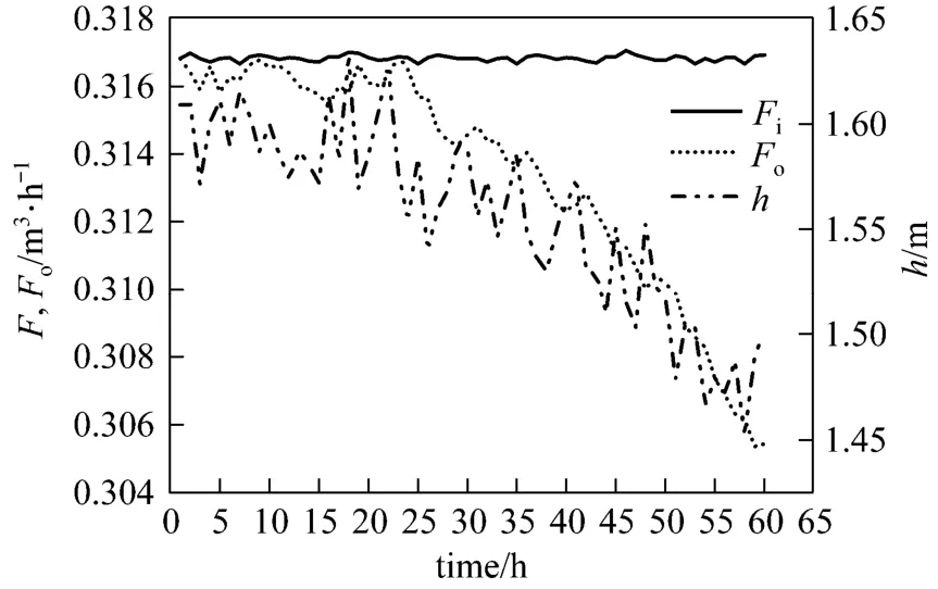
Figure 4 The data from measurement of tank system

3.4 Fault prediction model

In this section, the two methods depicted in Fig. 2 for hybrid fault prediction model are applied to the gravity tank example. After leakage occurs for 20 h, 40 measurement points about h and Foare collected with a sampling interval of 1.0 h. These data, spanning 40 h, constitute training set to build grey model and then time series model. The next 5 measurement points are collected to constitute testing set to verify fault prediction result.

3.4.1 The first prediction method

Two-variable grey model about h and Fois built with training set. After estimating its parameters using Eq. (9), the grey prediction model [Eq. (15)] changes to the following formula

40 measurement points about h and Foare predicted using Eq. (37). The prediction errors are shown in Fig. 5.

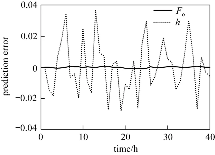
Figure 5 The error of grey prediction model

Figure 6 The value of BIC criteria function for time series model

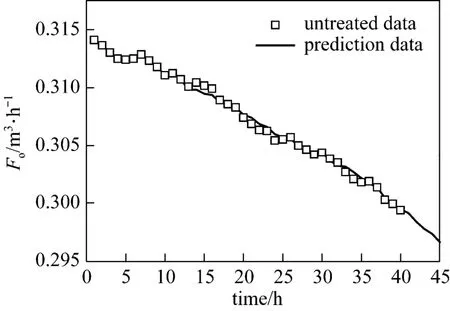
Figure 7 The simulation and prediction result of outlet flow rate

To build time series model with the prediction errors from the grey model, the order of prediction error of Foand h is first determined by the BIC criteria function. Fig. 6 gives the BIC value versus order and demonstrates a minimum BIC function value when the order is equal to 20. Thus 20 is chosen as the suitable order of time series model [Eq. (16)]. The coefficients in Eq. (16) are estimated by linear least square method and listed in Table 2. Eq. (16) with coefficients listed in Table 2 is combined with Eq. (37) to obtain the grey time series model about outlet flow rate [Eq. (38)] and liquid level [Eq. (39)] of tank. Figs. 7 and 8 depictsimulation result of the 40 measurement points and prediction result for the next 5 measurement points with Eqs. (38) and (39), respectively.

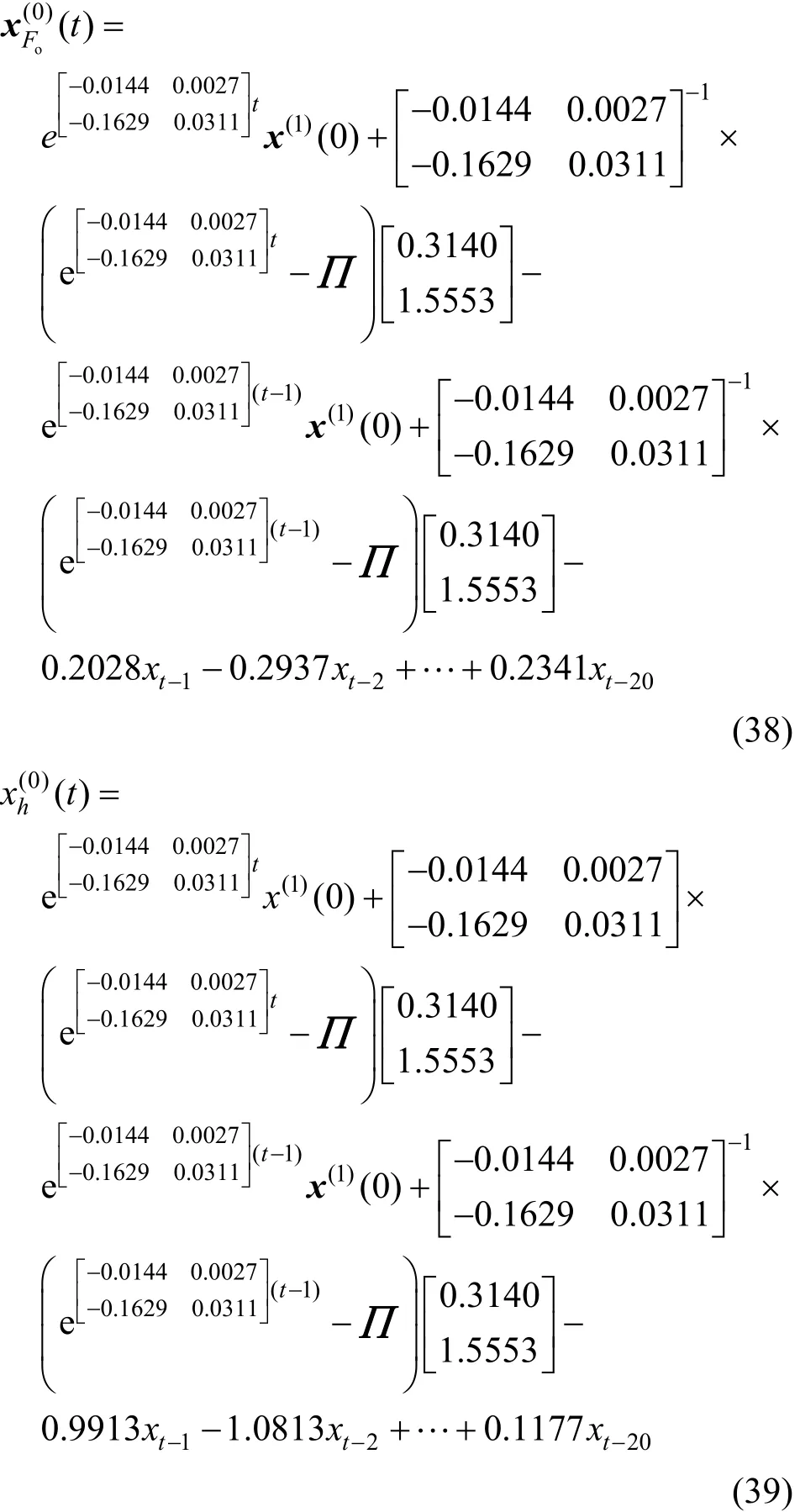
Table 2 Coefficient estimation of time series model

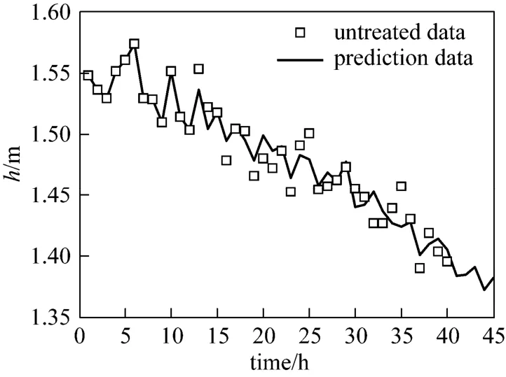
Figure 8 The simulation and prediction result of liquid level

The predicted 5 measurement points about h and Foare put into the dynamic tank model [Eqs. (29) to (32)] and then Cithat reflects leakage extent in entrance pipe are obtained through linear square method [Eq. (36)] and listed in Table 3, which shows that the first type of hybrid prediction model can predict fault parameter accurately.

Table 3 Predicted Ciusing the first method

3.4.2 The second prediction method

In this section, the second method depicted in Fig. 2 is applied in the gravity tank system. After leakage occurs in tank entrance for 20 h, 40 measurement points about h and Foare put into the dynamic model [Eqs. (29) to (32)], and then entrance flow rate coefficients Cifor these time points are calculated, shown as Fig. 9.

Figure 9 The calculated Cifor past 40 time points

Because only Cineeds to be predicted, singlevariable grey model is chosen. Using the value of Cigiven in Fig. 9 to get its coefficients, the grey model [Eq. (15)] becomes

Figure 10 contains the prediction error of Ciwith Eq. (40) for those 40 time points. The error value is put into the time series model [Eq. (16)] to determine its order with BIC function as criteria. Fig. 11 demonstrates the BIC value versus order, showing that BIC function is minimal when the order is equal to 20. Thus 20 is chosen as the suitable order of Eq. (16).

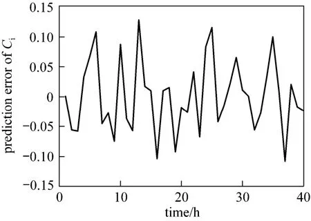
Figure 10 The prediction error of Ci with grey model with the second method

Figure 11 The value of BIC criteria function for time series model with the second method

The time series model with coefficients obtained by linear least square method is combined with the grey model to predict Ci. The grey time series model is

The values of Cirepresenting leakage extent in the past 40 and next 5 time points are calculated using Eq. (41), as shown in Fig. 12. Prediction error for the next 5 time points is listed in Table 4.

Figure 12 The simulation and prediction result of of Ci

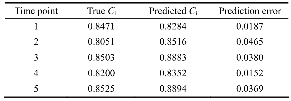
Table 4 Predicted Ciusing the second method

Table 4 shows that the second model also predicts fault parameters accurately. The difference between the two hybrid prediction models is specified by posterior variance test. Let S1and Si2be the variance of untreated data and prediction error, respectively. The ratio of posterior variance C is defined as

where i denotes prediction model index.

The ratio C is used to test prediction accuracy for these two methods. The data necessary for evaluation are listed in Table 5, which manifests that C1is less than C2, so the first method presents better prediction accuracy than the second one. Two reasons are behind such difference. The grey time series model amplifies the fault diagnosis error arising from dynamic model in the second method; the multi-variable grey model used in the first method is more accurate than the single-variable grey model used in the second method.

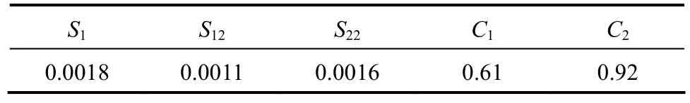
Table 5 Posterior variance test data

4 CONCLUSIONS

Grey model is combined with time series model in series to increase its adaptability to data oscillations for fault prediction. Further, the grey time series model is combined with dynamic model because the former is good at measurement prediction while the latter is good at fault parameter acquisition through fault diagnosis. Two combination methods for such hybrid fault prediction model are proposed and successfully implemented to predict entrance flow rate coefficient in a gravity tank system. The result shows that the first method is more accurate than the second one due to its control on dynamic model error and multi-variable grey model employed. Future research will focus on the application of the first method to large-scale systems.

NOMENCLATURE

REFERENCES

1 Venkatasubramanian, V., Rengaswamy, R., Yin, K., Kavuri, S.N., “A review of process fault detection and diagnosis Part I: Quantitative model-based methods”, Comput. Chem. Eng., 27, 293-311 (2003).

2 Min, H.K., Chang, K.Y., “Multivariate monitoring for time-derivative non-gaussian batch process”, Korean J. Chem. Eng., 25, 947-954 (2008).

3 Bin Shams, M.A., Budman, H.M., Duever, T.A., “Fault detection, identification and diagnosis using CUSUM based PCA”, Chem. Eng. Sci., 66 (20), 4488-4498 (2011).

4 Srinivasan, R., Qian, M.S., “Online fault diagnosis and state identification during process transitions using dynamic locus analysis”, Chem. Eng. Sci., 61 (18), 6109-6132 (2006).

5 Zheng, X.P., Liu, M.T., “An overview of accident forecasting methodologies”, J. Loss Prevent. Proc., 22 (4), 484-491 (2009).

6 Yoo, C.K., Kim, M.K., Hwang S.J., Jo, Y.M., Oh, J.M., “Online predictive monitoring and prediction model for a periodic process through multiway non-gaussian modeling”, Chin. J. Chem. Eng., 16 (1), 48-51 (2008).

7 Kim, M.J., Jiang, R., Makis, V., Lee, C.G., “Optimal Bayesian fault prediction scheme for a partially observable system subject to random failure”, Eur. J. Oper. Res., 214 (2), 331-339 (2011).

8 Suo, R.X., Wang, F.L., “The application of combination forecasting model in Chinese energy consumption”, Mathematics in Practice and Theory, 40 (18), 80-85 (2010).

9 Wu, Y.G., Zhu, X.F., Shi, B.H., “Control study of long time delay process based on grey predictive model”, Control Engineering of China, 14 (3), 278-280 (2007).

10 Wang, H.Z., Yang, J.P., Yu, N., “A fault prediction based on a grey nonlinear regression model”, Journal of Ordnance Engineering College, 22 (1), 46-48 (2010).

11 Wang, Z., Wang, Y., Zhang, J., “Grey correlation analysis of corrosion on oil atmospheric distillation equipment”, In: Proceedings of the 5th International Conference on Fuzzy System and Knowledge Discovering, Yin, Y.L., ed., IEEE, Jinan, China, 13-17 (2008).

12 Gao, D., Wu, C.G., Zhang, B.K., Ma, X., “Signed directed graph and qualitative trend analysis based fault diagnosis in chemical industry”, Chin. J. Chem. Eng., 18 (2), 265-276 (2010).

13 Zhang, X., Ma, S.L., Yan, W.W., Zhao, X., Shao, H.H., “A novel systematic method of quality monitoring and prediction based on FDA and kernel regression”, Chin. J. Chem. Eng., 17 (3), 427-436 (2009).

14 Lahiri, S.K., Ghanta, K.C., “Prediction of pressure drop of slurry flow in pipeline by hybrid support vector regression and genetic algorithm model”, Chin. J. Chem. Eng., 16 (6), 841-848 (2008).

15 Liu, S.F., Forrest, J., “The role and position of grey system theory in science development”, The Journal of Grey System, 9 (4), 351-356 (1997).

16 Hsu, C.C., Chen, C.Y., “Applications of improved grey prediction model for power demand forecasting”, Energ. Convers. Manage., 44 (14), 2241-2249 (2003).

17 Mao, M.Z., Chirwa, E.C., “Application of grey model GM(1, 1) to vehicle fatality risk estimation”, Technological and Social Change, 73 (5), 588-605 (2006).

18 Tian, W. D., Sun, S.L., “On-line dynamic model correction based fault diagnosis in chemical processes”, The Chinese Journal of Process Engineering, 7 (5), 952-959 (2007).

19 Tian, W.D., Guo, Q.J., Sun, S.L., “Dynamic simulation based fault detection and diagnosis for distillation column”, Korean J. Chem. Eng., 29, 9-17 (2012).

20 Isermann, R., “Model-based fault detection and diagnosis—Status and application”, Annual Reviews in Control, 29, 71-85 (2005).

21 Zhang, Z.D., Hu, S.S., “A new method for fault prediction of model-unknown nonlinear system”, Journal of the Franklin Institute, 345 (2), 136-153 (2008).

22 Frank, P.M., Ding, S.X., Marcu, T., “Model-based fault diagnosis in technical processes”, Transactions of the Institute of Measurement and Control, 22 (1), 57-101 (2000).

23 Li, R.Y., Rong, G.Z., “Fault isolation by partial dynamic principal component analysis in dynamic process”, Chin. J. Chem. Eng., 14 (4), 486-493 (2006).

24 Wang, Z.F., Yuan, J.Q., “Online supervision of penicillin cultivations based on rolling MPCA”, Chin. J. Chem. Eng., 15 (1), 92-96 (2007). 25 Chiang, L.H., Russel, E.L., Braatz, R.D., “Parameter estimation”, In: Fault Detection and Diagnosis in Industrial Systems, China Machine Press, Beijing, 179-189 (2003).

2013-08-13, accepted 2013-11-13.

* Supported by the Shandong Natural Science Foundation (ZR2013BL008).

** To whom correspondence should be addressed. E-mail: tianwd@qust.edu.cn