CO2Leakage Identification in Geosequestration Based on Real Time Correlation Analysis Between Atmospheric O2and CO2*

MA Denglong (马登龙), DENG Jianqiang (邓建强)and ZHANG Zaoxiao (张早校),**State Key Laboratory of Multiphase Flow in Power Engineering, Xi’an Jiaotong University, Xi’an 70049, ChinaSchool of Chemical Engineering and Technology, Xi’an Jiaotong University, Xi’an 70049, China

CO2Leakage Identification in Geosequestration Based on Real Time Correlation Analysis Between Atmospheric O2and CO2*

MA Denglong (马登龙)1,2, DENG Jianqiang (邓建强)2and ZHANG Zaoxiao (张早校)1,2,**
1State Key Laboratory of Multiphase Flow in Power Engineering, Xi’an Jiaotong University, Xi’an 710049, China2School of Chemical Engineering and Technology, Xi’an Jiaotong University, Xi’an 710049, China

The paper describes a method for monitoring CO2leakage in geological carbon dioxide sequestration. A real time monitoring parameter, apparent leakage flux (ALF), is presented to monitor abnormal CO2leakage, which can be calculated by atmospheric CO2and O2data. The computation shows that all ALF values are close to zero-line without the leakage. With a step change or linear perturbation of concentration to the initial CO2concentration data with no leakage, ALF will deviate from background line. Perturbation tests prove that ALF method is sensitive to linear perturbation but insensitive to step change of concentration. An improved method is proposed based on real time analysis of surplus CO2concentration in least square regression process, called apparent leakage flux from surplus analysis (ALFs), which is sensitive to both step perturbation and linear perturbations of concentration. ALF is capable of detecting concentration increase when the leakage occurs while ALFs is useful in all periods of leakage. Both ALF and ALFs are potential approaches to monitor CO2leakage in geosequestration project. Keywords CO2monitor, carbon storage, gas leakage, O2/CO2exchange, correlation analysis

1 INTRODUCTION

Carbon capture and sequestration (CCS) is considered for reduction of increase rate of atmospheric CO2. In CCS project, geological storage of CO2is one of the most promising options for carbon mitigation [1-9]. While the purpose of geologic carbon sequestration is to trap CO2underground, CO2could migrate away from the storage site into the shallow subsurface and atmosphere because of permeable pathways such as well bores or faults [7, 8]. Due to the negative impacts of CO2leakage on the sequestration and near-surface environment, it is suggested that the leakage should be monitored as a critical part in geologic carbon sequestration. Many techniques are available to measure near-surface CO2, such as gas chromatograph [10], seismic monitoring [11, 12], eddy covariance (EC) method [13, 14], soil gas sampling [13], tracer gas [15], and carbon stable isotopes measurement [16], but it is very difficult for most of these methods to detect abnormal condition in time and obtain leakage flux simultaneously due to the large difference in CO2fluxes and concentrations of natural background, within which a small CO2anomaly may be hidden.

Fessenden et al. [17] designed an O2/CO2measurement system to identify CO2subsurface seepage. They used long-term atmosphere monitor data before and during injection to compute and compare the variation of O2/CO2ratio between the two periods. However, it may be a problem that the O2/CO2ratio is regarded as a constant in the whole monitoring period because the ratio varies diurnally and seasonally. Therefore, a real-time monitoring method and a quantified evaluation parameter for CO2leakage flux are necessary for CO2geosequestration.

The main purpose of this study is to develop a real-time monitor model to detect CO2leakage in geosequestration based on O2/CO2ratio measurement and present a real time assessment parameter, apparent leakage flux (ALF), which is calculated from atmospheric O2and CO2concentrations, to estimate the CO2seepage and leakage.

2 DISPERSION OF LEAKAGE CO2FROM GEOSEQUESTRATION

In order to study the character of leakage CO2perturbation to the background CO2in atmosphere, the unsteady state atmosphere dispersion of leakage CO2from geosequestration is simulated by computational fluid dynamics [16, 18, 19], Fluent 13.0.

The leakage rate is assumed to be 1000 tons per year. A 3-D model is built within the distance of 200.0 m downwind (x direction), 50.0 m crosswind (y direction, y=0 is the midline) and 10.0 m height above the ground (z direction). The leakage CO2disperses over the bare soil surface and roughness height is 0.0 m. The wind speed is 5.0 m·s−1. Fig. 1 shows the dispersion at 100.0 m downwind along the midline at 1.5 m above the ground. The concentration increases with time at the beginning of leakage and gets to a peak concentration at some time, and then decreases so slightly that the concentration can be treated as a stable value. Therefore, the trend of concentration caused by leakage can be considered as a step perturbation of concentration relative to the background variation. In the initial stage of dispersion, the concentration increases.

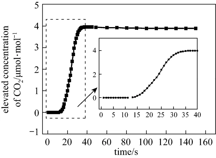
Figure 1 Unstable dispersion of leakage CO2at 100 m downwind along the midline at 1.5 meter above the ground (wind speed: 5 m·s−1; atmospheric stable length: 13 m)

3 MEASUREMENT OF O2/CO2RATIO

The variation of background CO2in the air is very complex, which is affected by moisture, temperature, barometric pressure, solar insulation, vegetations, fossil-fuel burning and so on [20, 21], so it is very difficult to detect the leakage CO2. It may be a feasible way to solve this problem by analyzing the relationship between CO2and O2in the air.

O2and CO2exchange ratio (−ΔO2/ΔCO2) is typically equivalent to one mole O2per mole CO2approximately as expected for respiration or photosynthesis. The main factors that produce different ratios are fossil-fuel burning and air-sea exchange [22-24]. When the ocean uptake is neglected in short period and smaller spatial scales, sinks and sources of O2and CO2mainly involve two processes, fossil-fuel burning and biomass metabolism including respiration and assimilation, which can be expressed as

where H2CO represents the approximate composition of biomass or organic matter. O2is consumed and CO2is produced in respiration process and inversely in photosynthesis [22, 25]. For aerobic respiration, m=1; for anaerobic respiration, m=0. The soil respiration and decay of organic matter in the soil should be considered though they are very small. As this process is reversible, the exchange ratio of O2and CO2is stabilized around 1. Assimilation and respiration fluxes from the terrestrial biosphere are assumed to have an O2/CO2exchange ratio of about 1.1 [26, 27].

The fuel burning process consumes O2and produces CO2,

Figure 2 Schematic of sinks and sources of O2and CO2in a system between terrestrial ecosystem and atmosphere

where x represents the type of fuel [22]. This irreversible process increases CO2in atmosphere but reduces O2. The exchange ratio of O2and CO2depends on the oxidative ratio of organic materials, varying from about 1.1 for coal to 2.0 for methane [22, 27].

Consequently, sources and sinks of CO2are inversely coupled to those of O2via their exchange ratios. Therefore, combined observations of atmospheric O2and CO2will give more information on carbon fluxes than that from CO2measurements alone.

Figure 2 shows an air box model, with sources and sinks of O2and CO2in a system between atmosphere and terrestrial ecosystem without considering air-sea exchange [27]. It is a simple model for a column of well-mixed canopy air. Horizontal advection of air is neglected. The net fluxes of O2and CO2in the system can be calculated. Here, Ffand Fb(mol·m−2·s−1) are CO2fluxes in fuel burning process and biomassmetabolism process. Rfand Rbare exchange ratios of O2to CO2in the two processes. With the leakage, a leakage flux (Fl) will be added in the model.

Without CO2leakage, the fluxes into and out of the box are from net assimilation, respiration of plant and soil, and net burning. Transient changes in CO2and O2in the air box are calculated from following mass balance as expressed in Eq. (3) and Eq. (4).

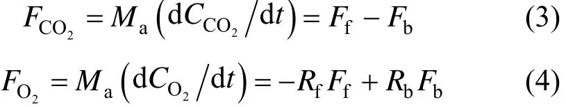
where Ma(mol·m−2) is moles of dry air per unit ground area,2COC and2OC (μmol·mol−1) are mole fractions of CO2and O2in an air box of specified height from the soil surface,2COF and2OF are net fluxes (mol·m−2·s−1) of CO2and O2in the air box.

Combining Eqs. (3) and (4), we have

where S0is a background ratio, which is a complex function of several environmental processes and is affected by many factors, such as soil moisture and temperature, and daily variation in solar insulation. However, if only terrestrial ecosystem is considered without air-sea exchange, the ratio in short time interval can be considered as constant because of relatively stable biomass metabolism process and less variable fuel composition.

4 APPARENT LEAKAGE FLUX

For a geological sequestration project in the terrestrial ecosystem as shown in Fig. 2, a CO2leakage flux, Fl, is added into the air box model. The leakage will change the net flux of CO2in the system but not that of O2. As a result, the transient change in CO2becomes

The transient O2/CO2ratio is changed to

where S is the current ratio, with a leakage flux added in the denominator compared with Eq. (5), which will decrease the ratio if the leakage occurs. With Eqs. (5) and (7), we have

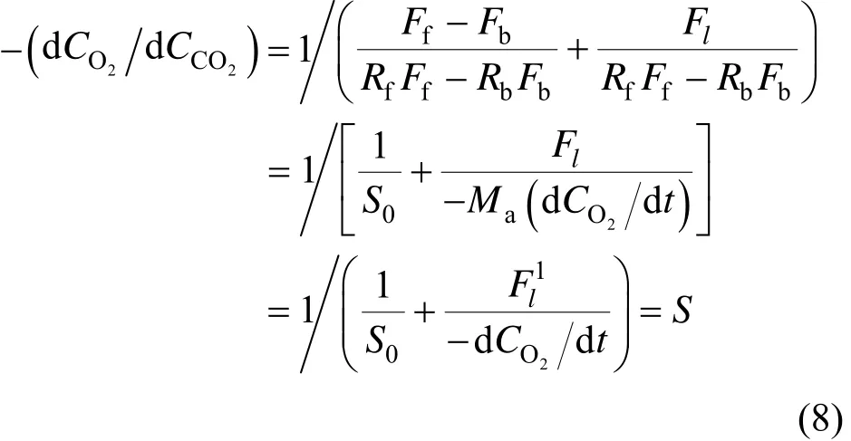
where Fl′=(Fl×106)/Ma(μmol·mol−1·s−1or ppm·s−1). BothlF andlF′ are defined as the apparent leakage flux (ALF).

Finally, a calculation equation for ALF is obtained

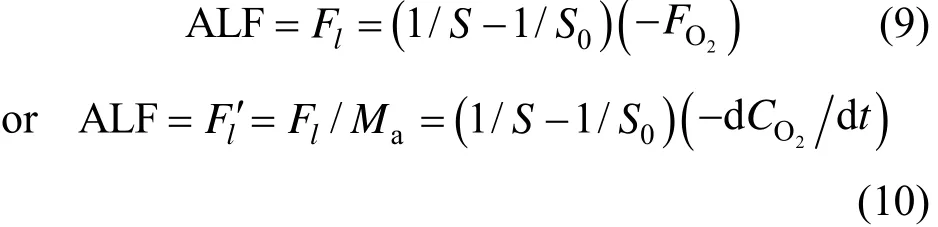
Equations (9) and (10) are composed of two parts. The first part (1/S−1/S0) represents the difference of O2/CO2ratio with and without leakage. Under normal circumstance,

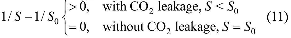
Because the direction of net O2flux is always opposite to the net CO2flux in ecosystem, the second part (−dCO2dt or −FO2) reflects the trend of CO2variance in the environment.

The unit of ALF in Eq. (9) is mol·m−2·s−1, the amount of leakage CO2per unit area per unit time. It may be obtained by flux measurement, such as EC method, which is not only a direct, in situ measurement, but also has much larger spatial scale (m2-km2) than other ground-based techniques [28]. The unit of ALF in Eq. (10) is μmol·mol−1·s−1, representing the amount of CO2accumulation, which characterizes CO2leakage indirectly and can be obtained by simple atmospheric O2and CO2monitoring.

When applying the ALF method to monitor leakage signals, the sensors should be located at downwind positions from potential leakage sources. More sensors will give more opportunities to detect leakage. However, when EC monitor instruments are used, the monitor area is mainly dependent on the height of monitor tower and much fewer sensors are required. Complex computation algorithms have to be designed when the EC tower is applied.

5 RESULTS AND DISCUSSION

5.1 Real-time leakage flux

Because S0and S cannot be calculated simultaneously, it is impossible to obtain the apparent leakage flux by directly applying Eq. (9) or Eq. (10). However, S0can be predicted using the data in previous time interval and S can be calculated by the data in current time interval. A recursion equation is

The first term in the parenthesis is current variation rate in current time step and the second term is the background value in the previous time interval, which are both computed by least square regression (LSR) method. The variation rate of O2concentration with time (dCO2dt) can be also calculated with LSR method.

Figure 3 Diurnal trend of concentrations of oxygen and carbon dioxide (a) and O2/CO2ratio (b)

Figure 4 Correlation of atmospheric O2and CO2concentrations for all day (a), daytime (b) and nighttime (c) (slope of line—exchange ratio)

The relative mole fraction data of atmospheric O2and CO2, measured on 25 and 26 October 1986 in Cambridge, Massachusetts, by Keeling [22], are used to test our real-time CO2leakage method.

5.2 Relative concentration of atmospheric O2and CO2

Figure 3 shows mole fractions of CO2and O2and the real time O2/CO2exchange ratio. Ambient CO2increases from 350 μmol·mol−1to 410 μmol·mol−1overnight while O2decreases by a similar amount. The O2/CO2ratio is close to 1 in most of time.

In order to obtain the correlation between O2and CO2, mole fraction data for all day, daytime and nighttime are selected (Fig. 4). The data yield linear relationship, with slopes close to 1.1, which represent the O2/CO2exchange ratio. It is higher during daytime (1.1288) and lower during nighttime (1.0261) because of stronger photosynthesis. At night, photosynthesis stops, and the variation of exchange ratio is mainly from biomass respiration and soil respiration.

5.3 Real-time apparent leakage flux

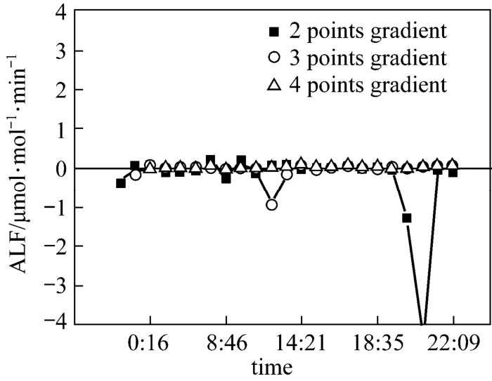
Figure 5 Real-time apparent leakage flux with different intervals

Figure 5 shows the apparent leakage flux calculated by Eq. (12) with the data of every two, three and four time intervals separately to estimate the background O2/CO2ratio S0in Eq. (10). With more previous points,the prediction is more precise. Without CO2leakage, the apparent leakage fluxes are all close to zero when S0is predicted with four interval data. The daily average ALF is 0.0057 μmol·mol−1·min−1and the average correlation coefficient of CO2to O2is 0.85.

Figure 6 Apparent leakage flux with concentration perturbation at distance 30 m

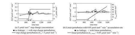
Figure 7 Apparent leakage flux with concentration perturbation at distance 50 m

5.4 Apparent leakage flux with CO2concentration perturbation

Based on the dispersion simulation of leakage CO2in Section 2, we assume that the leakage perturbation is a step change or a linear change of concentration, which is added to the initial CO2concentration with no leakage, to study the sensitivity of apparent leakage flux to leakage, and then the real time ALF without and with perturbations are computed. The perturbation functions are as follows

where Fst(μmol·mol−1) is a step change perturbation function and Flinear(μmol·mol−1) is a linear perturbation function, both are accumulated quantity.

According to the dispersion simulation results, the step change of concentration Cst(μmol·mol−1) in Eq. (13) is specified as 10 μmol·mol−1·min−1[Fig. 6 (a)], and the linear accumulation rate kc_linear(μmol·mol−1·min−1) in Eq. (14) is 0.1μmol·mol−1·min−1[Fig. 6 (b)] when measurement distance is 30 m, while Cstis 5 μmol·mol−1·min−1[Fig. 7 (a)] and kc_linearis 0.05 μmol·mol−1·min−1[Fig. 7 (b)] at the distance of 50 m.

ALF deviates from background base-line when a concentration perturbation is added to the initial data with no leakage. The response to the step change perturbation appears in a short period after the perturbation is added (t0) and the abnormal condition disappears rapidly (tf). The average ALF is 0.0086 μmol·mol−1·min−1with 5 μmol·mol−1· step change perturbation and it is 0.0090 μmol·mol−1·min−1with 10μmol·mol−1step change perturbation, while the average ALF of base line is 0.0057 μmol·mol−1·min−1. For linear perturbations, abnormal ALF occurs after the perturbation is added (t=800 min) and retains a certain period. The average ALF with linear perturbation of 0.05 μmol·mol−1·min−1accumulation rate is 0.0470 [Fig. 7 (b)], which is about 8 times that of base line. Therefore, ALF is sensitive to linear perturbation but insensitive to step change perturbation. The reason is that step change perturbation affects the surplus variables in real time linear regression process but not O2/CO2ratio except at t0, while linear perturbation affects O2/CO2ratio during all test time. In order to detect abnormal condition better, average values with every five interval ALF data are computed with 0.01, 0.03, 0.05, 0.08, and 0.1 μmol·mol−1·min−1accumulation rate, as shown in Fig. 8. The real time average ALF gives more significant results than that of single ALF monitoring. Table 1shows the error analysis with different linear accumulation rates. The relative error is less than 20% when accumulation rate is lower than 0.05 μmol·mol−1·min−1. It is more accurate with lower rate (less than 0.05 μmol·mol−1·min−1). Thus, ALF method is useful to detect the leakage at the initial linear increase stage.

Negative values of ALF in Figs. 6 and 7 may be resulted from unstable background O2/CO2ratio and imperfectly synchronous variation in CO2with O2. The atmospheric data used here may also affect the results. However, the results provide evidence that real time ALF is a potential method to monitor CO2leakage in geosequestration.

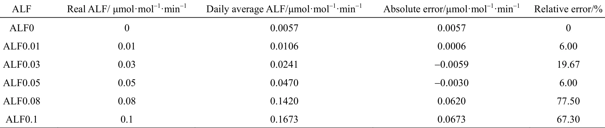
Table 1 Error analysis of ALF with different linear accumulation rates

Figure 8 Average apparent leakage flux with different linear perturbations

5.5 Improved ALF method

Above analysis shows that the variation of CO2in ecosystem is in a good linear relationship with the change of O2, but leakage perturbation will break this relation. According to Eqs. (5) and (7), the relationship between atmosphere CO2and O2in short time scales can be expressed as

whereBC andBC′ are the surplus concentrations of CO2in atmosphere during different time step, which have no linear correlation with O2. Eq. (15) is the background concentration in previous time step and Kiand Ki′+1, in real time LSR process. It is understandable that the surplus variablesB,tC andB,1tC+′ in real time LSR process will be affected in the same level with linear perturbation. On the other hand, the step change perturbation will only affect surplus variables but not the slopes except a short period after perturbation. These conclusions will be proved as follows.

For two sets of data (Xi, Yi), LSR is used for fitting [29]. In a linear estimation expression formula Eq. (16) is the current concentration in present step. In the computation process, they are calculated by the surplus variable in real time LSR process.

ALF can be used to detect the linear increasing perturbation, which corresponds to the variation of slopes, timated slopes, and βˆ is the estimated surplus variable. βˆ1and βˆ0can be calculated by

Yˆiis the predicted value of Yivariable,ˆ is the es-

step, and n is the number of calculation steps. When a perturbation variable C is added to Yi, the independent variable becomes Yi′= Yi + C . 1

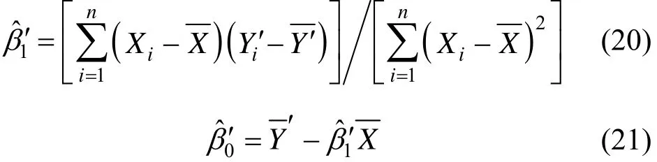
where 1 ˆβ′ and 0 ˆβ

′ are estimated slope and surplus variable with perturbation C, respectively. For linear perturbation C, C = C0i , where C0 is a constant, 1 ˆβ becomes

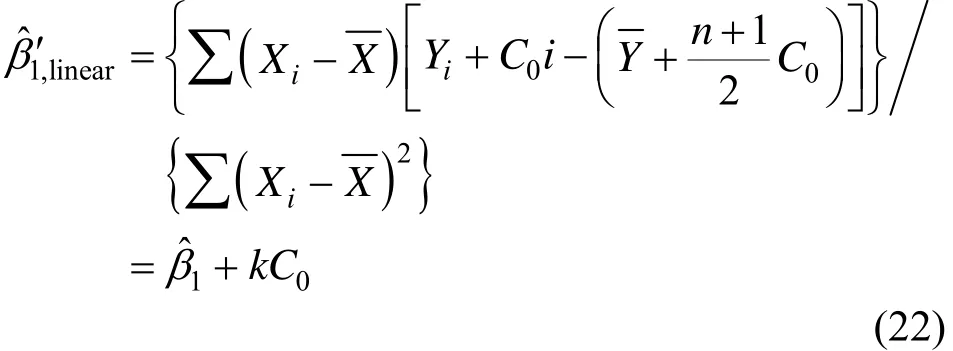
When Eqs. (22) and (24) are adopted for monitoring CO2leakage with CO2and O2linear correlation analysis, it is the ALF method. When Eqs. (23) and (25) are used, it is the apparent leakage flux from surplus analysis (ALFs),

In the ALF method, leakage rate is calculated directly, while in the ALFs method elevated concentration is obtained indirectly.

In order to test the sensitivity of ALFs method to the linear perturbation, accumulation rates are set as 0.01, 0.03, 0.05, 0.08, and 0.1 μmol·mol−1·min−1. The results are shown in Fig. 9. The ALFs calculated from surplus CO2concentration is able to detect the linear perturbation and the slope of the increasing part reflects the leakage rate. With the step change perturbations 3, 5, 10, and 20 μmol·mol−1added, as shown in Fig. 10, ALFs also responds to the perturbation. The overall trend can be viewed as a step change variation response. The perturbation concentration can be calculated by subtracting background concentration from the surplus CO2concentration.

Figure 9 Average ALFs with different linear concentration perturbations (accumulation rate: from 0.01 to 0.1 μmol·mol−1·min−1)

Figure 10 Average ALFs with different step change perturbations

The error analysis of ALFs to the perturbations is summarized in Table 2. The relative error of ALFs to linear perturbation is lower than 20% when the accumulation rate is larger than 0.01 μmol·mol−1·min−1, while the error is lower than 7% when accumulation rate is larger than 0.03 μmol·mol−1·min−1. Higher excessive accumulation rate decreases the error. Comparison of Tables 1 and 2 shows that the relative error of ALFs is lower than that of ALF with higher accumulation rate (>0.05 μmol·mol−1·min−1). Moreover, the relative error of ALFs to concentration perturbation is lower than 2% in all step change perturbations, while increasing step change concentration will reduce the error.

According to the above analysis, the ALFs method is sensitive to both linear and step change perturbations, whose application in CO2leakage monitoring is more extensive than ALF method.

6 CONCLUSIONS

A real time CO2leakage assessment parameter, ALF, is presented based on atmospheric oxygen and carbon dioxide monitoring. Without leakage, all ALF values are close to background zero-line, while they will deviate from the zero-line with concentrationperturbation. ALF is sensitive to linear perturbation but insensitive to step change of CO2concentration. The relative error of average ALF is less than 20% when test accumulation rate is lower than 0.05 μmol·mol−1·min−1.

An improved method, ALFs, is proposed by real time surplus CO2concentration calculated in LSR process. It is sensitive to both linear and step change perturbations. The relative error of ALFs to linear perturbation is less than 7% when the accumulation rate is larger than 0.05 μmol·mol−1·min−1, while it is lower than 2% in all tests with step change perturbations.

Both ALF and ALFs are potential methods to monitor CO2leakage in geosequestration project. They can identify the leakage from complex background variation in real time. The ALF is able to detect the leakage in concentration increasing stage, while the ALFs is useful in whole period of leakage.

However, these methods cannot determine the real leakage flux and locate leakage source at the same time, which will be our further work. We will improve this method and test it in the laboratory and field experiment.

Table 2 Error analysis of ALFs with linear and step change perturbations

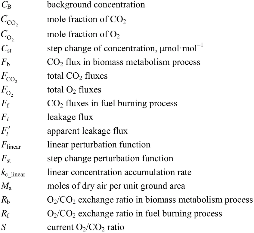
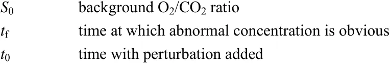
NOMENCLATURE

REFERENCES

1 Mao, J.F., Wang, B., Dai, Y.J., “Sensitivity of the carbon storage of potential vegetation to historical climate variability and CO2in continental China”, Adv. Atmos. Sci., 26 (1), 87-100 (2009).

2 Yang, L., Yu, H.B., Wang, S.Q., Wang, H.W, Zhou, Q.B., “Carbon dioxide captured from flue gas by modified ca-based sorbents in fixed-bed reactor at high temperature”, Chin. J. Chem. Eng., 21 (2), 199-204 (2013).

3 Ye, C.B., Chen, G.W., Yuan, Q., “Process characteristics of CO2absorption by aqueous monoethanolamine in a microchannel reactor”, Chin. J. Chem. Eng., 20 (1), 111-119 (2012).

4 Yu, Y.S., Li, Y., Lu, H.F., Yan, L.W., Zhang, Z.X., “Performance improvement for chemical absorption of CO2by global field synergy optimization”, Int. J. Greenh. Gas. Con., 5 (4), 649-658 (2011).

5 Yu, Y.S., Li, Y., Lu, H.F., Dong, R.F., Zhang, Z.X., “Synergy pinch analysis of CO2desorption process”, Ind. Eng. Chem. Res., 50 (24), 13997-14007 (2011).

6 Yu, Y.S., Liu, W.Q., An, H., Yang, F.S., Wang, G.X., Feng, B., Zhang, Z.X., Rudolph, V., “Modeling of the carbonation behavior of a calcium based sorbent for CO2capture”, Int. J. Greenh. Gas. Con., 10, 510-519 (2012).

7 Geng, J.H., Dong, L.G., Ma, Z.T., “Ocean bottom nodes time-lapse seismic survey for monitoring oil and gas production and CO2geological storage”, Adv. Earth Sci., 26 (6), 670-676 (2011). (in Chinese)

8 Dong, H.S., Huang, W.H., “Research of CO2capture, geological storage and leakage technologies”, Resour. Ind., 12 (2), 123-128 (2010). (in Chinese)

9 Lewicki, J.L., Hilley, G., Oldenburg, C., “An improved strategy to detect CO2leakage for verif i cation of geologic carbon sequestration”, Geophys Res. Lett., 32 (19), L19403 (2005).

10 Wang, Y.S., Wang, Y.H., “Quick measurement of CH4, CO2and N2O emissions from a short-plant ecosystem”, Adv. Atmos. Sci., 20 (5), 842-844 (2003).

11 Prestona, C., Monea, M., Jazrawi, W., Lawf, D., Chalaturnykg, R., Rostronh, B., “IEAGHG Weyburn CO2monitoring and storage project”, Fuel. Process. Technol., 86 (14), 1547-1568 (2005).

12 Hilke, W., Fabian, M., Michael, K., Heidugd, W., Christensene, N.P., Borma, G., Schilling, F.R., “CO2SINK—From site characterization and risk assessment to monitoring and verif i cation: One year of operational experience with the fi eld laboratory for CO2storage at Ketzin, Germany”, Int. J. Greenh. Gas. Con., 4, 938-951 (2010).

13 Lewicki, J.L., Fischer, M.L., Hilley, G.E., “Six-week time series of eddy covariance CO2flux at Mammoth Mountain, California: Performance evaluation and role of meteorological forcing”, J. Volcanol. Geoth. Res., 171 (3), 178-190 (2008).

14 Liu, H.P., “A re-examination of density effects in eddy covariance measurements of CO2fluxes”, Adv. Atmos. Sci., 26 (1), 9-16 (2009). 15 Ray, L., David, E., Ashok, L., Bronwyn, D., “Atmospheric monitoring and verif i cation technologies for CO2geosequestration”, Int. J. Greenh. Gas. Con., 2 (3), 401-414 (2008).

16 John, D.A., Computational Fluid Dynamics: The Basics with Applications, McGraw-Hill Education, USA (1995).

17 Fessenden, J.E., Clegg, S., Rahn, T., Humphries, S., Baldridge, W.,“Novel MVA tools to track CO2seepage, tested at the ZERT controlled release site in Bozeman. MT”, Enviro. Earth. Sci., 60 (2), 325-334 (2010).

18 Hanna, S.R., Briggs, G.A., Hosker, R.P., Handbook on atmospheric diffusion, USA Department of Energy, Tech. Inf. Cent., USA, DOE/TIC-11223 (DE82002045) (1982).

19 Ma, D.L., Deng, J.Q., Zhang, Z.X., “Numerical study on unsteady state dispersion of leakage CO2from geological sequestration”, J. Xi’an Jiaotong Univ., 46 (9), 102-107 (2012). (in Chinese)

20 Zhao, M., Pitman, A.J., “The relative impact of regional scale land cover change and increasing CO2over China”, Adv. Atmos. Sci., 22 (1), 58-68 (2005).

21 Klusman, R.W., “Comparison of surface and near-surface geochemical methods for detection of gas microseepage from carbon dioxide sequestration”, Int. J. Greenh. Gas. Con., 5, 1369-1392 (2011).

22 Keeling, R.F., “Measuring correlations between atmospheric oxygen and carbon dioxide mole fractions: A preliminary study in urban air”, J. Atmos. Chem., 7, 153-176 (1988).

23 Keeling, R.F., Najjar, R.P., Bender, M.L., Pieter, P.T., “What atmospheric oxygen measurements can tell us about the global carbon cycle”, Global. Biogeochem. Cy., 7 (1), 37-67 (1993).

24 Keeling, R.F., Manning, A.C., Manvendra, K.D., “The atmospheric signature of carbon capture and storage”, Philos. T. Roy. Soc. A, 369 (1943), 2113-2132 (2011).

25 Manning, A.C., “Temporal variability of atmospheric oxygen from both continuous measurements and a flask sampling network: Tools for studying the global carbon cycle”, Ph.D. Thesis, Univ. Calif., San Diego, USA (2001).

26 Severinghaus, J.P., “Studies of the terrestrial O2and carbon cycles in sand dune gases and in Biosphere”, Ph.D. Thesis, Columbia Univ., New York, USA (1995).

27 Seibt, U., Brand, W.A., Heimann, M., Lloyd, J., Severinghaus, J.P., Wingate, L., “Observations of O2︰CO2exchange ratios during ecosystem gas exchange”, Global Biogeochem Cycl., 18, GB4024, 1-18 (2004).

28 Lee, X., Massman, W., Law, B., Handbook of Micrometeorology, Kluwer Academic Publishers, Netherlands (2004).

29 Graybill, F.A., Iyer, H.K., Regression Analysis: Concepts and Applications, Duxbury Press, Belmont, California, USA (1994).

2013-04-08, accepted 2013-06-07.

* Supported by the National Natural Science Foundation of China (51276141, 20936004).

** To whom correspondence should be addressed. E-mail: zhangzx@mail.xjtu.edu.cn