Numerical simulation of turbulent flow around a forced moving circular cylinder on cut cells*

BAI Wei

Department of Civil and Environmental Engineering, National University of Singapore, Singapore 117576, Singapore, E-mail: w.bai@nus.edu.sg

Numerical simulation of turbulent flow around a forced moving circular cylinder on cut cells*

BAI Wei

Department of Civil and Environmental Engineering, National University of Singapore, Singapore 117576, Singapore, E-mail: w.bai@nus.edu.sg

(Received December 26, 2012, Revised August 4, 2013)

Fixed and forced moving circular cylinders in turbulent flows are studied by using the Large Eddy Simulation (LES) and two-equation based Detached Eddy Simulation (DES) turbulence models. The Cartesian cut cell approach is adopted to track the body surface across a stationary background grid covering the whole computational domain. A cell-centered finite volume method of second-order accuracy in both time and space is developed to solve the flow field in fluid cells, which is also modified accordingly in cut cells and merged cells. In order to compare different turbulence models, the current flow past a fixed circular cylinder at a moderate Reynolds number, =Re3 900, is tested first. The model is also applied to the simulation of a forced oscillating circular cylinder in the turbulent flow, and the influences of different oscillation amplitudes, frequencies and free stream velocities are discussed. The numerical results indicate that the present numerical model based on the Cartesian cut cell approach is capable of solving the turbulent flow around a body undergoing motions, which is a foundation for the possible future study on wake induced oscillation and vortex induced vibration.

Cartesian cut cell, turbulent flow, Large Eddy Simulation (LES), Detached Eddy Simulation (DES), forced oscillating cylinder

Introduction

In parallel with the development of offshore engineering extending towards the deeper water and harsher environment, the investigation of fluid interaction with flexible slender members has already attracted considerable attention, due to the extensive existence of this problem in different situations, such as marine risers, mooring lines, spars, cables etc. In addition, this kind of slender members always appears in the form of clusters. Therefore, the wake shielding effect must be taken into account in determining the response of the member clusters. Generally speaking, the flexible member in clusters will experience the Wake Induced Oscillation (WIO) in the streamwise direction controlling if the members collide or not, and the Vortex Induced Vibration (VIV) in the spanwise direction, respectively.

Over the last few decades, significant progress has been made in understanding the VIV of a long circular cylinder by means of both the numerical simulation and the physical experiment. The recent development of VIV can be found in the review article by Williamson and Govardhan[1]. However, the investigation of WIO of a downstream circular cylinder is relatively behind the study of VIV, probably because of the large motion that the downstream cylinder suffers which could make the investigation much more difficult. The previous research on WIO thus mainly focused on the model measurement, for example, Okajima et al.[2]studied the streamwise oscillation of two tandem circular cylinders in a wind tunnel, and Sagatun et al.[3]measured the acceleration and impulsive force of the downstream cylinder and indicated the phenomenon of collision between two adjacent cylinders.

On the other hand, the numerical investigations of flow interaction with a moving circular cylinder were always carried out in two dimensions, due to the unaffordable computational effort required in 3-D simulations. Among those available publications on this topic, Prasanth et al.[4]studied the laminar flowinduced vibration of a circular cylinder at low Reynolds numbers, and Wanderley et al.[5], Al-Jamal and Dalton[6]adopted the RANS and LES turbulence models to simulate the VIV response at moderate Reynolds numbers respectively. At the same time, studies have been extended to the case of two circular cylinders, and emphasis has been put on the shielding effect of upstream cylinder on the laminar flow induced motion of downstream one, such as Prasanth and Mittal[7]and Papaioannou et al.[8]where the latter implemented the unstructured triangular mesh and the mesh regeneration was required in order to track the body motion.

From the above discussion, it may be observed that all the previous works used the body-fitted grid to discretize the computational domain in which one or two bodies are moving around. Therefore, in principle, mesh regeneration must be performed at every time step, which is time-consuming for some certain grid types. For the bodies undergoing a large amplitude motion, some mesh regeneration techniques will fail or large numerical error will occur on some undesirable coarse meshes. In addition, due to the movement of the grid, interpolation technology is also required to predict the values of variables on the new grid. It should be noted that the interpolation might cause some numerical errors, depending on the interpolation technology adopted. These attributes of the body-fitted grid provide the motivation for the present work. In this paper, the flow field is simulated on a fixed structured Cartesian cut cell grid.

The present paper is a direct extension of the numerical method presented by Bai et al.[9], where a cell-centered Finite Volume Method (FVM) based on a structured Cartesian cut cell grid with a colocated variable arrangement has been developed for the analysis of 2-D laminar flows with and without free water surface. Here, different turbulence models, including the Smagorinsky-type Large Eddy Simulation (LES) model and thekω- based Detached Eddy Simulation (DES) model are introduced into this well-developed algorithm to deal with the turbulent flows. These turbulence models are verified and evaluated by comparing with the experimental data for the flow past a fixed circular cylinder at =Re3 900. This paper focuses on the investigation of a forced oscillating circular cylinder in turbulent flows, which is expected to be a firm foundation for the possible future study on freely moving cylinders with a very large displacement appearing in WIO and VIV problems.

It should be mentioned that the forced oscillating cylinder has been studied recently by Atluri et al.[10], where the vorticity-stream function equations in the cylindrical coordinates has been used, but its extension and application in complex bodies with arbitrary large motions may be much limited by the numerical method they adopted. In addition, Lin[11]also developed a numerical model on a fixed background grid for the simulation of a moving body in free surface flows, in which a so-called openness function was defined in each cell to represent the fraction of volume of solid phase in this cell. We can see that the representation of the body in his method seems to be fuzzy, whereas the present cut cell approach can define the position of body surface clearly and precisely because we just adopt the body boundary to “cut” the background grid behind. Therefore, the cut cells include the accurate information of the boundary surface rather than a representation by a percentage fraction, which may have direct influence on the accuracy of the results.

1. Mathematical formulation

Both LES and RANS turbulence models are employed to study the flows around fixed and moving bodies. Although their mechanism of production is quite different, with time averaging in RANS and spatial filtering in LES, in both cases the governing equations can be casted into a general form on a Cartesian coordinatesix, where =i1 or 2 for a horizontal 2-D flow considered here, whereiuis the averaged or filtered velocity in the RANS and LES turbulence models respectively,ρandνare the density and the kinematic viscosity of the fluid, andpdenotes the pressure. All unresolved effects of turbulence are absorbed into the Reynolds stressijτ, and different closure models forijτwill lead to different turbulence models.

1.1Smagorinsky LES turbulence model

The most widely used LES turbulence model is the Smagorinsky Sub-Grid Scale (SGS) model. Although it was initially proposed for 3-D turbulent flows, it has been applied to simulate 2-D flows with reasonable successes. In this LES model, the unknown subgrid stress tensor can be represented by

whereνTis the eddy viscosity andSij=(∂ui/∂xj+∂uj/∂xi)/2 is the strain rate tensor of the large scaleor resolved field. Furthermore, a simple algebraic formula is employed to determine the eddy viscosity

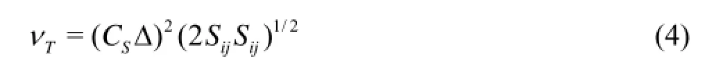
whereSCis the Smagorinsky constant and Δ is the characteristic subgrid length scale given by the square root of the element area for 2-D cases. Commonly, the widely used value ofSCvaries from 0.1 to 0.3, and is chosen to be 0.1 here.

1.2kω-based DES model

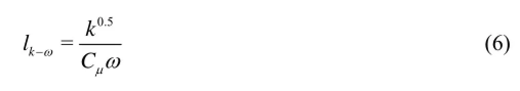
In order to obtain the model used in the DES formulation, the corresponding turbulence length scalelin the individual RANS turbulence model has to be predicted first. By comparing this length scale and the modified local grid spacing, a minimum value is taken and given to the DES length scaled,

This DES length scale will be adopted in solving the RANS type of turbulence equations in the DES model. In addition, ΔDES=max(Δx,Δy) for 2-D cases, where Δxand Δyare the grid sizes in thex- andy-directions respectively, andCDESis a constant of the DES turbulence model equal to 0.65 in the calculations. The aim of the DES model is to achieve a RANS simulation in the vicinity of walls and LES in areas of massive flow separation outside of the boundary layer. In this model, only the RANS type of turbulence equations are required to be solved without any explicit declaration of RANS versus LES zones. The change in the length scale leads to a model that becomes region-dependent in nature: in most cases a RANS model in the boundary layers and a LES model in separated regions. These advantages of the DES model can help to increase the efficiency of the numerical method significantly, because only the relatively coarser mesh is required in the boundary layer around the body surface, instead of a very fine mesh used in the LES model.

In the present paper, a populark-ωRANS model is adopted to construct the DES turbulence model, as it has some advantages over thek-εmodel in transitional flows and in adverse pressure gradient boundary layer flows. Furthermore, no any kind of damping function is required to extend the model to the near-wall region. In this model, an additional turbulence specific dissipation rateωis defined asω=ε/(Cμk), replacing the dissipation rateεin thek-εmodel. Here,kis the turbulent kinetic energy andCμis a constant equal to 0.09 here. Based on the definition ofω, the eddy viscosity can be predicted byνT=k/ω. Accordingly, the turbulence length scale for this model can be defined as

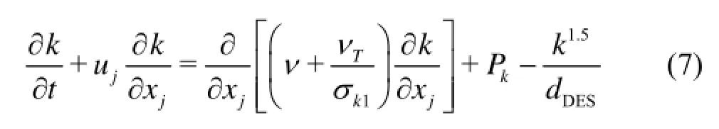
After comparing with the modified local grid size, the length scale of the DES modeldcan be predicted by Eq.(5). Consequently, the transport equation for the turbulent kinetic energykcan be rearranged, in conjunction with the length scale of the DES model obtained before,

The transport equation for the specific dissipation rateωremains unchanged in thekω- based DES turbulence model, and its standard expression is

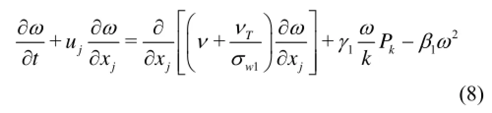
The model closure coefficients used for thek-ωturbulence model areσk1=2.0,σω1=2.0,γ1=0.553 andβ1=0.075.Pkdenotes the production of turbulent energy, which has the form ofPk=τij∂ui/∂xj=νT(2SijSij).

1.3Boundary conditions

Besides satisfying the governing momentum and continuity equations, the flow is also subject to various boundary conditions on all surfaces of the fluid domain. At the inlet boundary the fluid velocity is specified. At the outlet boundary, the condition should make the boundary “transparent”, i.e., the numerical solution in the inner computational region would not be affected by the outlet boundary. Here a periodic condition is introduced at the far field boundary for the purpose of simplicity, which is found to be effective as no obvious reflection has been detected in the numerical simulations. A Neumann-type boundary condition needs to be introduced for the pressure on all the boundary surfaces. On the solid body surfaces non-slip boundary conditions are applied. Here, the circular cylinder starts oscillating in the streamwise direction from its rest position, thus the displacement of its motionχis given aswhereωis the oscillation angular frequency andadefines the amplitude of body motions.

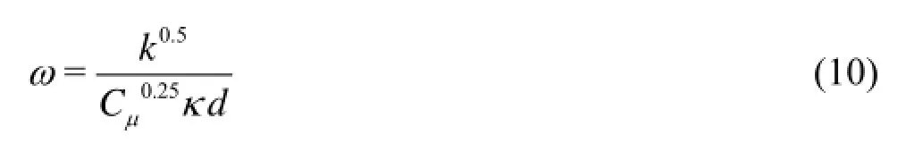
Furthermore, the boundary conditions also need to be set for various unknown turbulence variables. At all non-slip boundaries, the turbulent kinetic energy and the specific dissipation rate are all equal to zero, i.e.,k=ω=0. Since the problem is solved in the time domain, an initial condition must be imposed. In order to raise the speed of convergence, the free stream velocityu0at the inlet boundary is used to prescribe the fluid velocity within the whole domain. The turbulence variables are given a uniform value all over the domain ask=1×10-6u2andω=10k/ν. At the 0 same time, it is often assumed that the flow is in local equilibrium, which means the production and dissipation are nearly equal. Based on this approximation, the equation forωis not applied in the elements next to the wall, instead,ωat these elements is explicitly set equal to

2. Numerical model

A numerical solution to the Navier-Stokes equations has been developed by using a cell-centered Finite Volume Method (FVM) based on a Cartesian cut cell approach proposed by Bai et al.[9], where applications have been carried out for 2-D laminar flows with free water surfaces. The cut cell method produces a boundary conforming mesh without the necessity to make the boundary a coordinate surface. In fact, there is no mesh generation in the conventional sense; all that is necessary is to calculate the intersections of a series of line segments with a background Cartesian grid. Therefore, moving boundaries can be easily accommodated by re-computing cell-boundary intersections, rather than remeshing the whole flow domain or large portions of it. In practice, a cut cell can be arbitrarily small, numerical stability may be compromised at these small cut cells. To overcome this problem cell merging is implemented. If the fluid area in a cut cell is less than a certain percentage of the total cell area (here 10% is chosen as the critical value), this cut cell is considered to be a small merging cell, and it should be merged to a suitable neighboring cell based on a designed criteria. The total computational domain is composed of fluid cells, cut cells, solid cells, merged cells and small merging cells, as shown in Fig.1. Only fluid cells, cut cells and merged cells need to be treated separately; these will be discussed next.

For fluid cells, the momentum equation is discretized by the schemes of second-order accuracy, and the SIMPLE algorithm with a collocated variable arrangement is adopted to solve the pressure-velocity coupling, more details can be found in many textbooks, such as Ferziger and Perić[12]. For cut cells, the discretized equation is based on the same algorithm developed for fluid cells, with the non-slip boundary condition at the cut surface corresponding to the solid wall. However, when the neighbouring cell of a cut cell is a small merging cell (such as the top surface of the cut cell shown in Fig.1), a specific explicit treatment is used to avoid arranging unknowns on the small merging cell, because we do not wish to encounter a numerical instability issue. In this case, the small merging cell is regarded as a boundary cell with the known value from the previous iteration.

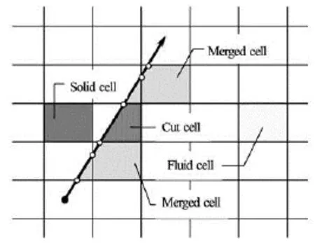
Fig.1 Sketch of definition for the cut cell mesh

For merged cells, the situation is more complex, because two neighboring cells may exist at one cell face of a merging cell (such as the bottom surface of the merged cells shown in Fig.1). When this situation happens, one neighboring cell is a fluid cell and the other one is a cut cell or a small merging cell. We can not treat both of them implicitly, otherwise, this would destroy the band structure of the resulting algebraic equation system. The approach here is to use the unknowns in the fluid cell and calculate the influence of the cut cell or the small merging cell explicitly.

From the above discussion, it is noticed that an iteration procedure as required by the SIMPLE algorithm is employed to predict the velocity and the pressure of the fluid at a certain time instant. When the LES turbulence model is chosen, at the end of each time instant, the eddy viscosity needs to be updated by using Eq.(4). While if the two-equation RANS based DES turbulence model is involved in the simulation, we have to solve two additional transport equations, Eqs.(7) and (8), which have the very similar formulation compared to the momentum equation in Eq.(2). Thus, the similar numerical schemes can be used to discretize the transport equations in the RANS model. In addition, in order to ensure the stability of the simulation, the turbulence transport equations need to be solved and the eddy viscosity is updated right after theflow field is determined in one iteration. Once the iteration is convergent, the velocity, pressure as well as other turbulence parameters will have the desired values at that time instant.

As was mentioned above that the cut cell approach can easily accommodate moving boundaries in the fluid domain, the extension of the numerical model to consider moving bodies here is straightforward. At each time instant, the new position of the body surface can be updated on the basis of the prescribed motion of the body, based on which the cell-boundary intersections can be re-computed. Therefore, the fluid cell, cut cell and merged cell can be re-defined for a new domain, and the computation can continue.

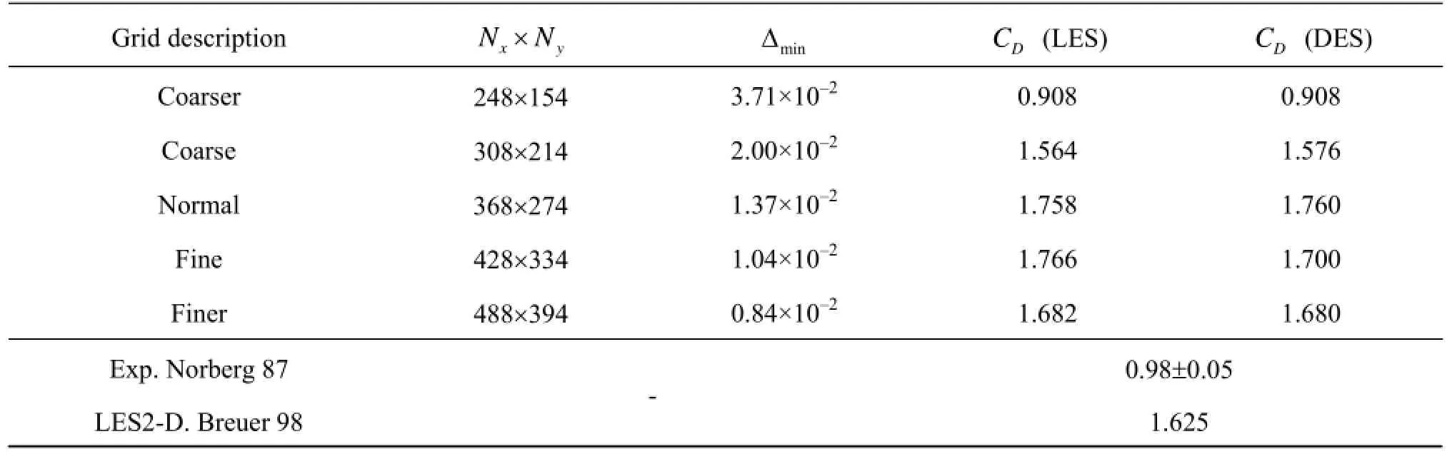
Table 1 Convergence of mean drag coefficient with different grids using LES andkω- based DES turbulent models for flow over a fixed circular cylinder at =Re3 900

3. Numerical results

3.1Validation by a fixed single cylinder

We first calculate the turbulent flow past a circular cylinder using different LES and DES turbulence models at =Re3 900 and compare the results with the published experimental and numerical data. Grid convergence tests are carried out with different non-uniform meshes. In this mesh system, the relatively coarser mesh is employed in the region far away from the body, while the finer mesh must be generated around the body surface. In addition, the fine mesh is also required in the wake behind the circular cylinder. Unless otherwise stated, the fluid density, free stream velocity and diameter of the cylinder are taken to be unity in all cases discussed below, yielding results and time in non-dimensional form. Other lengths are non-dimensionalized by the diameter of the cylinder.

Table 1 shows the numerical results of the drag coefficientDCobtained with five different meshes. In this table, the first two columns represent the numbers of elements in the -xand -ydirections, and the minimum grid size around the circular cylinder, respectively. The total simulating time is 300 for all these meshes. A small time interval taken as =tΔ0.5 that can satisfy the stable requirement even for the finer mesh remains the same for all the meshes, in order to assess the influence of various meshes only. It can be seen that the normal mesh can predict acceptable convergent results for both cases using two different turbulence models. From the comparison, the DES turbulence model and the LES model can provide quite close numerical results. With the consideration of efficiency, the LES model will be used in the next example. However, the DES model remains to be an option in the present numerical model.

However, the present drag coefficient seems to be out of the range of the experimental result obtained by Norberg[13], and this discrepancy is due to the neglect of the 3-D effect in the current 2-D simulation. In other words, the 2-D simulation always overestimates the drag coefficient at this Reynolds number. This point has also been noticed by another 2-D numerical simulation in Breuer[14], which is also included in Table 1. We find that the present drag coefficient is in reasonable agreement with his 2-D numerical result.

3.2Preliminary results of flow around a forced oscillating cylinder

Next, we investigate a circular cylinder undergoing forced oscillations at different amplitudes and frequencies at =Re2 000 in terms of the unit free stream velocity, which is a first step in simulating the freely moving riser cluster in ocean current and waves. A coarse mesh (defined as coarse mesh in Table 1) is adopted in the simulations, to save the computer time without losing the accuracy significantly. In some numerical examples, the total simulating time is shortened, because of the very small oscillation period of the forced motion that is dominant over the flow field. In addition, a smaller time interval is employed for some cases, depending on the oscillation frequency and amplitude where the oscillation frequency is the main limitation for the time interval. For example, forthe cylinder moving at =0.1ωπ and =a0.3 in a turbulent flow, the time interval is equal to 0.02, while the time intervals have to be set as 0.01 and 0.005 for cases at =0.4ωπ and =0.8ωπ respectively.

However, a new problem arises. Figure 2 shows the time history of the drag force on the cylinder undergoing a forced oscillation at =0.2ωπ and =a0.3. We can notice that the force is not varying smoothly, and it fluctuates around the mean value. The reason for this fluctuation is the use of merged cells. As the body is moving at every time step, the change of the cell type from cut cell to merged cell or reverse may occur; this process can not be avoided. When this process happens, some numerical errors would be introduced into the simulation, because we assume a uniform distribution of the variable over the merged cell. As it is known that the pressure is always convergent slower than the velocity, some time steps are required to eliminate this numerical error in the pressure. Therefore, the variation of the velocity is always smooth, but the force process involves many fluctuations as shown in Fig.2. One possible way to remove this fluctuation is to use the smoothing technique.

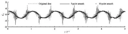
Fig.2 Drag coefficient on the forced moving cylinder at =0.2ωπ and =a0.3 and consequent results by different smoothing techniques

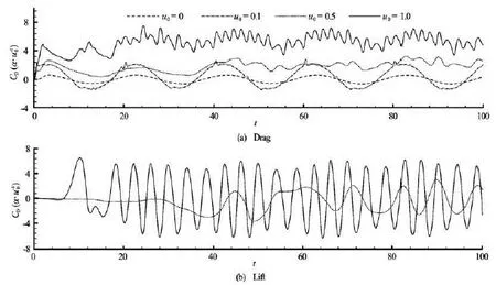
Fig.3 Force coefficients on the forced moving cylinder at =0.1ωπ and =a0.3 for different prescribed inlet velocities

The smoothing only can utilize the results obtained at the previous time steps, because the drag forces at the following time steps are still unknown at a specified time instant. We have tried to smooth the results by taking the average over the last 5 time steps and 10 time steps respectively, as denoted by 5-point smooth and 10-point smooth in Fig.2. It can be seen that this simple technique works well. The resulting curves using these two smoothing parameters are quite close, both of them are also in good agreement with the mean value of the drag force at each time step. After comprehensive comparisons, it is recommended that the average is performed overT/50-T/25, whereTis the oscillation period. It should be mentioned that the average over a too long period is not encouraged, because it will delay the phase of the results.

3.3Influence of free stream velocity

Next, we fix the motion of the cylinder at =ω0.1π and =a0.3 and place the cylinder in the turbulent flow with different free stream velocities,0=u0.1, 0.5 and 1.0 respectively. These free stream velocities correspond to =Re200, 1 000 and 2 000 respectively. However, in order to directly compare with the amplitude of the cylinder motion, the free stream velocity is adopted here as an indicating parameter, instead of the Reynolds number. It can be noticed that the Reynolds numbers considered here are not very large. The reason is that a relatively coarse mesh is adopted in this study, with the purpose of avoiding the expensive computational cost that may be caused by the finer mesh for higher Re numbers. The influence of the free stream velocity on the drag and lift coefficients can be observed in Fig.3, where the drag and lift coefficients are also multiplied by a parameter0/auifu0is unequal to 0, in order to consider the variation of the free stream velocity in the dimensionless force coefficients.

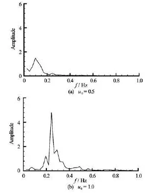
Fig.4 Amplitude spectra of lift coefficient on the forced moving cylinder at =0.1ωπ and =a0.3 for different prescribed inlet velocities

It should be noted from the figure that the mean drag force becomes larger with increasing the free stream velocity. At0=u0.1, the effect of the external flow is negligible, and the flow field is solely dependent on the forced body motion. While this effect becomes significant at0=u1.0, and the natural vortex shedding frequency governs the flow pattern more than the body motion frequency. As the external turbulent flow has dominated the flow pattern whenu0=1.0, it is reasonable to expect that the increase ofu0can further increase the importance of the external flow in the flow field, which certainly leads to the same flow pattern of the predominant external flow. It is known that in this case the natural vortex shedding period and the body motion period correspond to 4 and 20 respectively, but the period of the force coefficient atu0=0.5 is obviously neither one of these, which indicates that the flow experiences the transition phase, and the competition between these two frequencies occurs.

This phenomenon also can be pointed out in Fig.4, in which the amplitude spectrum of lift coefficient by means of the Fast Fourier Transformation (FFT) is plotted. Only one peak value can be found in both two cases ofu0=0.5 and 1.0. The peak value is identical to the natural vortex shedding frequency atu0=1.0. The peak frequency seems to be around 0.1 atu0=0.5, which is located between the natural vortex shedding frequency (0.25 approximately) and the body motion frequency (0.05 exactly).

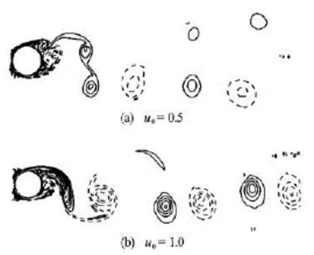
Fig.5 Instantaneous vorticity contour behind the forced moving cylinder at =0.1ωπ and =a0.3 for different prescribed inlet velocities

Figure 5 shows the flow pattern behind the forced oscillating circular cylinder for different free stream velocities. From the instantaneous vorticity contours, it can be observed that two rows of vortex street are generated, due to the motion of the body at0=u0.5. However, only one row of vortex street is remained for the larger free stream velocity at0=u1.0 which is quite similar to that for a fixed circular cylinder, because in this case the external turbulent flow dominates the flow field as discussed before.

3.4Influence of oscillation frequency

In order to investigate the influence of oscillation frequency on the results, we calculate the drag and lift coefficients on the circular cylinder oscillating with the amplitude of =a0.3 at four different frequencies:the results can be observed in Fig.6. For all these four cases, the free stream velocity is set to be 1.0, and the force coefficients are expressed in terms of the free stream velocity. The mean drag force is comparable for all these four cases, but the amplitude of the drag force has a big difference. Increasing the frequency, the amplitude of the drag force tends to increase at the same time. At smaller oscillation frequencies, this increase is not very obvious. Actually, the drag forces atω=0.1π and 0.2π are quite close. However, when the frequency increases from 0.4π to 0.8π, the trend of increase becomes very clear. The amplitude of the lift force is quite close for different cases. At the lower oscillation frequency, the flow pattern is governed by the external turbulent flow, while the effect of the body motion becomes stronger with the increase of the frequency, and finally dominates the drag force frequency atω=0.8π.

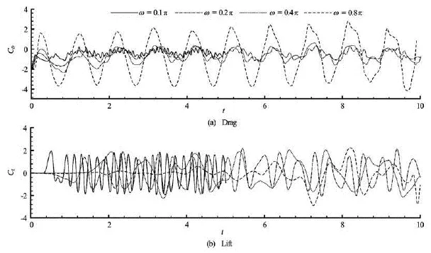
Fig.6 Force coefficients on the forced moving cylinder at =a0.3 and0=u1.0 with different oscillation frequencies

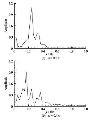
Fig.7 Amplitude spectra of lift coefficient on the forced moving cylinder at =a0.3 and0=u1.0 with different oscillation frequencies

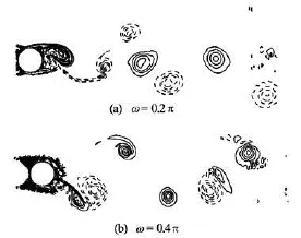
Fig.8 Instantaneous vorticity contour behind the forced moving cylinder at =a0.3 and0=u1.0 with different oscillation frequencies

The amplitude spectrum of lift coefficient for different oscillation frequencies is also shown in Fig.7. In conjunction with the result in Fig.4(b), we can see that at the lower frequency of =0.1ωπ, only onepeak frequency exists, corresponding to the natural vortex shedding frequency. However, with increasing the forced oscillation frequency to =0.2ωπ, two frequencies appear: one is the natural vortex shedding frequency, and the other is a higher-frequency nonlinear component, due to the nonlinear interaction between the natural vortex shedding frequency and the body motion frequency. This higher-order nonlinear component can also be found in Fig.7(b), where there are three peak frequencies in total. Besides this nonlinear component, the amplitude corresponding to the natural vortex shedding frequency decreases, and a new predominant frequency appears which is quite close to the body oscillation frequency, due to the stronger influence of the body motion in this case.

Figure 8 shows the instantaneous vorticity contour behind the cylinder oscillating at different frequencies. We can see from Fig.8(b) for =0.4ωπ that two rows of vortex street appear. Based on the comparison with Fig.5(b) where only one row of vortex street can be observed for =0.1ωπ, it may approach a conclusion that a body moving in a current always tends to induce two rows of vortex streets, even though sometimes these two rows of vortex streets can be supperssed and reduced to one row when the current is predominant in the flow field. At =0.2ωπ in Fig.8(a), this is a transition process between the phenomena at higher and lower frequencies.

3.5Influence of oscillation amplitude

At last, the body motion amplitude is increased, in order to ensure if the current numerical method can deal with the body undergoing large amplitude motions. The drag and lift coefficients on the body oscillating at =0.1ωπ,0=u1.0 are plotted in Fig.9. From the figure, we can notice that the variation tendency of the drag force is quite similar for both small and large amplitude motions, except that the amplitude of the oscillating force increases with increasing the body motion amplitude. This is because the body motion could destroy the regularity of the vortex shedding, which leads to a more unsteady flow field. In addition, the mean drag coefficient decreases a little due to the increase of the body motion. However, the amplitudes of the lift coefficients are close for these two cases.

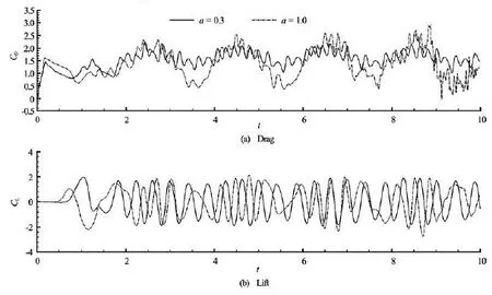
Fig.9 Force coefficients on the forced moving cylinder at =0.1ωπ,0=u1.0 with different motion amplitudes

4. Conclusion

The turbulent flow past fixed and forced moving circular cylinders has been solved by using a finite volume method based on the Cartesian cut cell approach. From the numerical examples presented here, it can be seen that the cut cell approach is particularly suitable for extending current flow solvers to investigate complicated moving boundary problems. The comparison of results for the turbulent flow around a fixed cylinder indicates that the current 2-D results are always overestimated, but in good agreement with others’ 2-D results. From the results of a cylinder undergoing forced oscillations at different frequencies and amplitudes, it can be seen that two rows of vortex streets appear when the body motion affects the flow field strongly. If the external turbulent flow is dominant, only one vortex shedding frequency occurs in the wake of the moving cylinder. With the increase of the body motion frequency, a higher-frequency nonlinearcomponent appears, and it retains its frequency even at the higher body oscillation frequency. When the body motion predominates the flow field, there are totally three frequencies competitive in the wake of the cylinder: the approximate body motion frequency, the natural vortex shedding frequency and the higherorder frequency.

[1] WILLIAMSON C. H. K., GOVARDHAN R. A brief review of recent results in vortex-induced vibrations[J].Journal of Wind Engineering and Industrial Aerodynamics,2008, 96(6-7): 713-735.

[2] OKAJIMA A., YASUI S. and KIWATA T. et al. Flowinduced streamwise oscillation of two circular cylinders in tandem arrangement[J].International Journal of Heat and Fluid Flow,2007, 28(4): 552-560.

[3] SAGATUN S. I., HERFJORD K. and HOLMAS T. Dynamic simulation of marine risers moving relative to each other due to vortex and wave effects[J].Journal of Fluids and Structures,2002, 16(3): 375-390.

[4] PRASANTH T. K., BEHARA S. and SINGH S. P. et al. Effect of blockage on vortex-induced vibrations at low Reynolds numbers[J].Journal of Fluids and Structures,2006, 22(6-7): 865-876.

[5] WANDERLEY J. B. V., SOUZA G. H. B. and SPHAIER S. H. et al. Vortex-induced vibration of an elastically mounted circular cylinder using an upwind TVD two-dimensional numerical scheme[J].Ocean Engineering,2008, 35(14-15): 1533-1544.

[6] AL-JAMAL H., DALTON C. Vortex induced vibrations using large eddy simulation at a moderate Reynolds number[J].Journal of Fluids and Structures,2004, 19(1): 73-92.

[7] PRASANTH T. K., MITTAL S. Flow-induced oscillation of two circular cylinders in tandem arrangement at low Re[J].Journal of Fluids and Structures,2009, 25(6): 1029-1048.

[8] PAPAIOANNOU G. V., YUE D. K. P. and TRIANTAFYLLOU M. S. et al. On the effect of spacing on the vortex-induced vibrations of two tandem cylinders[J].Journal of Fluids and Structures,2008, 24(6): 833-854.

[9] BAI W., MINGHAM C. G. and CAUSON D. M. et al. Finite volume simulation of viscous free surface waves using the Cartesian cut cell approach[J].International Journal for Numerical Methods in Fluids,2010, 63(1): 69-95.

[10] ATLURI A., RAO V. K. and DALTON C. A numerical investigation of the near-wake structure in the variable frequency forced oscillation of a circular cylinder[J].Journal of Fluids and Structures,2009, 25(2): 229-244.

[11] LIN P. A fixed-grid model for simulation of a moving body in free surface flows[J].Computers and Fluids,2007, 36(3): 549-561.

[12] FERZIGER J. H., PERIĆ M.Computational methods for fluid dynamics[M]. 3rd Edition, Berlin, Heidelberg: Springer, 2002.

[13] NORBERG C. Effects of Reynolds number and low-intensity free stream turbulence on the flow around a circular cylinder[R]. Publ. No. 87/2, Department of Applied Thermoscience and Fluid Mech., Chalmers University of Technology, Gothenburg, Sweden, 1987.

[14] BREUER M. Large eddy simulation of the subcritical flow past a circular cylinder: numerical and modeling aspects[J].International Journal for Numerical Methods in Fluids,1998, 28(9): 1281-1302.

10.1016/S1001-6058(13)60430-8

* Biography: BAI Wei (1973-), Male, Ph. D., Assistant Professor