On Propagation of Electromagnetic Waves in CylindricalWaveguides with Imperfectly Conducting Walls＊

LIN Qionggui

(School of Physics and Engineering,Sun Yat-sen University,Guangzhou 510275,China)

In classical electrodynamics,thesubjects of waveguides and resonant cavities are of practical importance.The physical theory for the subjects has been developed long ago and their applications have also been widely studied[1-7].Relevant subjects still attracted attentions in recent years[8-12].

The walls of waveguides are made of good conductors.They are treated as perfect ones in the lowest order approximation,since the solutions to the field equations are well known in this case.The effect of a finite conductivity is considered as a small perturbation to the boundary conditions.It leads to attenuation and shift of the wave number(propagation constant).The perturbative method for this problem has been formulated several decades ago[7].The formulation was then closely followed in the textbooks[1,4],andto our knowledge it was not further developed.

In this paper we present an improvement to the previous formulation[7].The general results are reformulated.The equation for calculating the corrected eigenvalues is obtained in a quite different for m.For mulas for calculating corrections to the eigenfields are given as well.Though the equation that determines the corrected eigenvalues obtained here is substantially equivalent to the previous one,several advantages are gained in the present for m:it is physically more transparent,formally simpler and more compact,and more convenient for practical calculations.Subtlety of spe-cial cases that was overlooked previously is analyzed and modifications to the general formulation are presented.It turns out that results for these special cases can be obtained from those for the ordinary case by a limit process.Therefore for practical calculations the special cases need not be treated separately.We also give the corrected eigenvalues for the coaxial line,which seems not available in the literature.

First we briefly review some general results and the previous for mulation[7].Consider a cylindrical waveguide with a generatrix parallel to the zaxis,and an arbitrary cross section which occupies a two-d imensional region Don thexy plane.The boundary ofDis denoted by∂D.The region Dmay bemultiply connected,for which the coaxial line is a typical example.The guide is filled with a dielectric medium whose permeability isμand permittivity is∈.All other parts of the space are filled with a conductor which has a permea bilityμc,permittivity∈cand conductivityσ.The propagating electromagnetic waves in the guide have the for m

whereρstands for the coordinates on thexyplane.We use the same symbolEfor the fieldE(x,t)andE(ρ),and similarly for the magnetic field.This would not lead to confusion since we will mainly useE(ρ)andH(ρ)in the following.W ith the transverse-longitudinal decomposition

where^kis a unit vector along thezaxis,ande(ρ)and h(ρ)are transverse fields,we have the field equations

whereΔtis the transverse gradient operator acting onρ.

In the ideal case when the walls are perfect conductors,we have T M,TE and TEM(ifDis multiply connected)modes.For practical calculations,it is convenient to solve the longitudinal fields first and obtain the transverse ones from Eqs.(3b)and(3d).The problems are

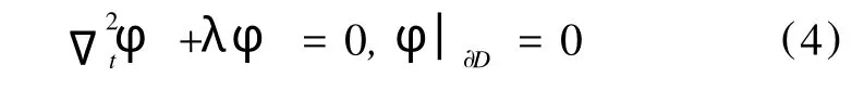
for T M modes and

for TE modes,where∂ψ/∂n=n·Δtψandnis a unit vector nor mal to∂Dand points in the inward direction,and

The TEM mode(only onemodeifDis doubly connected)corresponds toλ=0.It has no longitudinal fields and has to be solved individually.In general the spectrum for Eq.(4)and that for(5)is different.All eigenvalueswill be denoted by(the superscript 0 indicates that these are eigenvalues for the ideal case),in the order that 0=<<<…….Corresponding to an eigenvaluethere existdα(a positive integer)independent modes indicated by the subscripts α(=1,2,……,dα).Asαjalways followsαitwill be s imply denoted by.jThe field components for the modeαjare{φαj,eαj,ψαj,hαj},whereψαj=0 if it is a T M mode andφαj=0 if it is TE,and both vanish if it is TEM.They are related to one another by Eq.(3)whereλ=andk=[is related toby Eq.(6)].Theφαjwith differentαare automatically orthogonal and those with the sameαbut differentjare chosen to be orthogonal,and similarly forψαj.We do not normalize them.

For theoretical treatment,itmay be more convenient to deal with the transverse electric fielde,which in the ideal case satisfies

The solutionswill be denoted byεαj.These are essentiallyεαj∝Δφtαjfor T M modes andεαj∝k^×for TE modes,and some TEM onesε0j.According to the above convention they satisfy the orthogonal condition

We do not normalize them.All these solutions for m a complete set of vector functions in the regionD.The difference betweenεαjandeαjshould be remarked.In general we can identifyeαjwithεαj.However,if the frequencyωis such thatω2μ∈=for someγ,then for T Mγjmodes(if any)eγjvanishes and the set{eαj}is not complete in these cases.On the other hand,εγjdoes not vanish and the set{εαj}is always complete,but in the above special casesεγjis not a component of the physical fields so that the relation(3)is not appli-cable to it.In Ref.[7],the perturbed transverse fieldewas expanded in terms ofεαj(in our notations).This is correct.However,in subsequent discussions on the result for non-degenerate eigenvalues,relations like(3)were used,where the subtlety of the above special caseswas overlooked.Therefore the previous formulation left spaces for improvement.On the one hand,in the general result everything was expressed in terms ofεαjso that the advantages of the current formulation is absent.On the other hand,when relations like(3)were used to s implify a specific result,modifications to the general for mulation that may be necessary were not discussed.

Now consider the case when the walls are good but not perfect conductors.The field equations are still the above ones but we have the pertur bative boundary condition at∂D[1]

where the subscript‖indicates the components parallel to the boundary surfaces,andis the skin depth of the conductor.From this it can be shown that

In Green's identity for vector functions[4]

where dsis the arc element of the boundary,using the field equations foreandeαjand the boundary conditions for the latter,it is easy to obtain

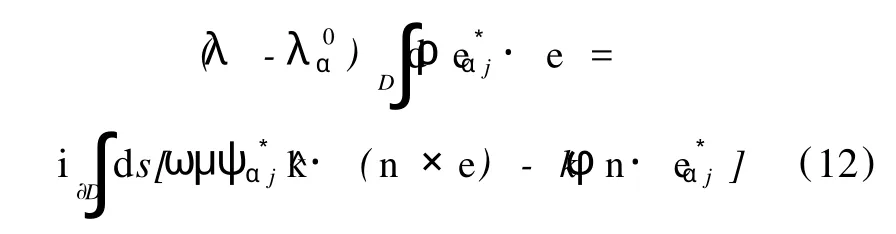
Substituting the boundary condition(10)into it,we have

This is the starting point for approximate calculations of the perturbed eigenvalues and fields.Ref.[7]began with a result similar to this and employed zero-order expansion of the eigenfields,thus corrections to the eigenfieldswere not discussed there.We will improve the general formulation in the following and calculate the corrected eigenfields aswell as the corrected eigenvalues.

We temporarily assume that the frequencyωis such thatω2μ∈is not equal to any,then the set{eαj}can be identified with{εαj}and is complete,so we have the expansion

According to Eq.(3)we have

Substituting these into Eq.(13)and using the orthogonal relation(8)we obtain

This can be simplified as follows.If theαjth mode is T M,it can be shown that

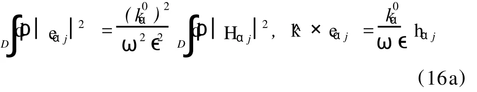
if it is TE or TEM,we have

W ith these relations and note thatψαj=0 in the first case,Eq.(15)can be recast into the form

This is the simplified and symmetrized[though equivalent to Eq.(13)]starting point for approximate calculations of the perturbed eigenvalues and fields.It is an eigenvalue problem for the eigenvalueλand the eigenvector represented by the set{aαj}.Because it is a system of homogeneous linear equations,the eigenvalueλis determined by the condition that the deter minant of the coefficient matrix should vanish.Note that we do not nor malize the eigenfield so that one coefficient in the set{aαj}is arbitrary for a given mode.

Equation(17)involves an infinite number of var-iables and exact solutions are not available.For good conductorsδis very small compared with the length scale ofD,so thatwe can approximately solve it in an iterative way.In the lowest order(zero-order)approximation,δ→0,so we have theνth(ν=0,1,2,...)solution

where the nonvanishing coefficientsare arbitrary at this order and have to be deter mined at the next order.Substituting theνth solution into the right-hand side(rhs)of Eq.(17),we obtain

This is the starting point for calculating theνth solution to the first-order,accordinglyλon the left-hand side(lhs)has been replaced by.Forα=νthe coefficientsaνjon the lhs are(still unknown),while forα≠νtheaαjare(this is similar to the stationary perturbation theory in quantum mechanics).Therefore forα=νwe have the eigenvalue equation in theνth subspace

This determines the first-order approximate eigenvalueand the corresponding zero-order fields.Afterandaν(l0)are obtained,Eq.(19)forα≠νgiveswhich determine the first-order correction to the eigenfield of theνth solution.

Equation(20)is the main result of this paper.In comparison with the corresponding equation in Ref.[7],it has several advantages.First,we know that the correction is due to the effective surface current and the finite conductivity,and the surface current is proportional to the magnetic field on the boundary surface.The rhs of Eq.(20)exhibits this physical origin definitely.It also shows that the longitudinal and the(tangential)transverse components of the magnetic field play the same role.Therefore the current result gives a clearer physical picture.Second,Eq.(20)is formally much simpler and more compact.This is obvious.Third,since only the magnetic fields are involved it is more convenient for practical calculations.

Let us make some more remarks.First,though Eq.(20)is valid only for the first-order eigenvalues,higher-order corrections are not of much significance because the boundary condition(9)itself is approximate.Second,the above for mulation has to be modified whenωis such thatω2μ∈=λ0γ,however,we will see below that Eq.(20)is still valid in this case.Third,let

whereuis a dimensionless parameter,then Eq.(20)can be written in the for m

Since the matrix Misobviously Her mitian,we immediately draw the conclusion thatuis real.This is not obvious in the previous for mulation.In special cases where

which happens for the square guide,the circular guide and the coaxial line,thejth solution is simply

whereNjis a constant.For circular guides and coaxial lines,the degeneracy between TE0n(one mode)and T M1n(two independent modes)is removed by the perturbation,while the degeneracy between the two independent modes of T Mmn(m≠0,the T M0nis non-degenerate)is not,and similarly for TEmn.This conclusion is in fact a nonperturbative one that can be achieved by studying the exact solutions.For the circular guide thiswas studied previously[3,8].

Now we turn to the special cases whenω2μ∈=(γis afixed positive integer).In this case alleαjcan be identified withεαjexcept for T Mγj(if any)whosevanishes.Even though all theγjmodes are TE,the above formulation has to be modified since these modes have=0 which renders some of the above for mulas trivial ormeaningless.

For the T Mγjmodeswe take

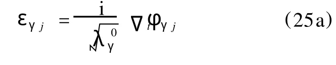
then the field components other thanφγjare

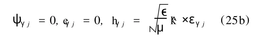
For the TEγjmodeswe have

where the subscripts are still those described before,the tilde is used just to emphasize that they are TE modes.In the current case Eq.(14a)should be modified as

where the second summation is over all T Mγl(the coefficients are changed tocγl)and the third over all TEγl,and the prime in the first summation indicates thatβ≠γ.Accordingly to Eqs.(3),(25)and(26),we have

The basic equation(13)is still valid.However,for the T Mγjmodes it becomes trivial.In this case it is replaced by the following one which can be obtained by s imilar derivations.

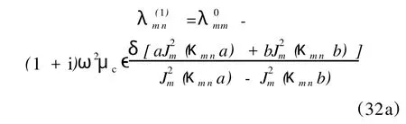
Similar to Eq.(17),the following results can be worked out.

These appears somewhat complicated,but the consequences that follow are not.By analysis similar to that following Eq.(17),the correction toλν(whereν≠γ)is still determined by Eq.(20),but the first-order correction to the eigenfields has a somewhat different for m.On the other hand,the correction toλγis determined by

Ifwe write these equations in a matrix form,the matrix is of a block triangular form,so that the determinant depends only on the two diagonal blocks.Therefore it is convenient to solve for the eigenvalue.

Itmay appear somewhat unpleasant that the above special cases need a separate treatment.However,lettingcoefficient in Eq.(25a)we haveεγj]in Eq.(17)and working out thecarefully(the crucial point is thatψγj=0 is exactwhile.it turnsout that the results are nothing other than Eq.(29).S imilarly,Eq.(20)forν=γreduces to Eq.(30)under the same condition.Therefore,for practical calculations,one just deals with the ordinary case,and results for the special cases can be produced by taking the corresponding limit.The process does not involve much subtlety and the rectangular guide serves as a simple example for verification of this point.The unpleasant issue is thus removed.

Finally we calculate the corrected eigenvalues forcoaxial lines.It seems that only the result for TEM[note thatwith the choice of wave was given in the literature[3].The inner and outer radii of the coaxial line are a and brespectively.We do not use the above convention for subscripts.In the ideal case,the eigenvalues for T M modes arewhereκmnis thenth(n=1,2,...)positive root of

The degeneracy of the corrected eigenvalues has been mentioned before.The corrected results form=0 andcan also be obtained by studying the exact solutions and solving the exact eigenvalue equation approximately.Form≠0,however,the exact eigenvalue equation is unexpectedly complicated and we have not been able to solve it.

In conclusion,Eqs.(20)and(19)for the correction of eigenvalues and eigenfields,respectively,are valid for any frequency.Though the progressmade in this paper ismainly a fo rmal one,it gives a clearer physical picture for the problem,clarifies some subtle point,makes calculationsmore convenient and may be beneficial to practical applications.

[1] JACKSON J D.Classical electrodynamics[M].3rd ed.New York:W iley,1998.

[2] GUO S H.Electrodynamics[M].3rd ed.edited by HUANGN-B,L I Z-B,L IN Q-G.Beijing:Higher Education Press,2008.(in Chinese)

[3] STRATTON J A.Electromagnetic theory[M].New York:McGraw-Hill,1941.

[4] COLL IN R E.Field theory of guided waves[M].New York:McGraw-Hill,1960.

[5] GOUBAU G.Electromagnetic waveguides and cavities[M].New York:Pergamon,1961.

[6] ARGENCE E,KAHAN T.Theory of waveguides and cavity resonators[M].London:Blackie and Son,1967.

[7] PAPADOPOULOS V M.Propagation of electromagnetic waves in cylindricalwave-guideswith imperfectly conductingwalls[J].Quart J Mech Appl Math,1954,7(3):326-334.

[8] ABE T,YAMAGUCH I Y.Propagation constant below cutoff frequency in a circular waveguide with conducting medium[J].IEEE Trans Microw Theory Tech,1981,29(7):707-712.

[9] DING R,TSANG L,BRAUN ISCH H.Wave propagation in a randomly rough parallel-plate waveguide[J].IEEE Trans Microw Theory Tech,2009,57(5):1216-1223.

[10] SCHÜZHOLD R,UNRUH W G.Hawking radiation in an electromagnetic waveguided[J].Phys Rev Lett,2005,95(3):031301.

[11] L IN Q G.Nonperturbative solutions to cylindrical resonant cavities with dissipative medium and imperfectly conducting walls[J].Chin Phys B,2010,19(1):010302.

[12] CHEN Xiaowen,L IU Yexin,WU Tianhong,et al.A-nalysis of stripe waveguide with the three-dimensional scalar finite-difference time-domain method[J].Acta Scientiarum Naturalium Universitatis Sunyatseni,2005,44(3):119-121.