Global patterns and ecological drivers of taxonomic and phylogenetic endemism in angiosperm genera

Hong Qian ,Brnt D.Mishlr ,Jian Zhang ,Shnhua Qian

a Research and Collections Center,Illinois State Museum,1011 East Ash Street,Springfield,IL 62703,USA

b University and Jepson Herbaria,Department of Integrative Biology,University of California,Berkeley,CA 94720-2465,USA

c Center for Global Change and Complex Ecosystems,Zhejiang Tiantong Forest Ecosystem National Observation and Research Station,School of Ecological and Environmental Sciences,East China Normal University,Shanghai 200241,China

d Shanghai Institute of Pollution Control and Ecological Security,Shanghai 200092,China

e Key Laboratory of the Three Gorges Reservoir Region's Eco-Environment,Ministry of Education,Chongqing University,Chongqing 400045,China

Keywords: Angiosperm Current climate Endemism Historical climate change Topographic heterogeneity

ABSTRACT Endemism of lineages lies at the core of understanding variation in community composition among geographic regions because it reflects how speciation,extinction,and dispersal have influenced current distributions.Here,we investigated geographic patterns and ecological drivers of taxonomic and phylogenetic endemism of angiosperm genera across the world.We identify centers of paleo-endemism and neo-endemism of angiosperm genera,and show that they are mostly located in the Southern Hemisphere in tropical and subtropical regions,particularly in Asia and Australia.Different categories of phylogenetic endemism centers can be differentiated using current climate conditions.Current climate,historical climate change,and geographic variables together explained～80% of global variation in taxonomic and phylogenetic endemism,while 42-46%,1%,and 15% were independently explained by these three types of variables,respectively.Thus our findings show that past climate change,current climate,and geography act together in shaping endemism,which are consistent with the findings of previous studies that higher temperature and topographic heterogeneity promote endemism.Our study showed that many centers of phylogenetic endemism of angiosperms,including regions in Amazonia,Venezuela,and west-central tropical Africa that have not previously been identified as biodiversity hotspots,are missed by taxon-based measures of endemism,indicating the importance of including evolutionary history in biodiversity assessment.

1.Introduction

Species richness and composition vary greatly among regional floras across the world (Rosenzweig,1995;Qian et al.,2023).One important measure is the degree of endemism in a region.Endemism reflects how speciation,extinction,and dispersal have influenced species distributions,and thus lies at the core of understanding the variation in community composition among regions(Qian,2001;Sandel et al.,2020).The concept of endemism is central to ecology,conservation biology,and biogeography (Crisp et al.,2001).Conservation biologists are interested in centers of endemism because of their importance in conservation given that small-ranged species are potentially threatened (Linder,1995;Myers et al.,2000),while biogeographers are interested in areas of endemism because they reflect the results of evolutionary and ecological processes (e.g.,speciation,extinction,and dispersal) in generating variation in species composition among regions(Anderson,1994;Brown and Lomolino,1998).

Traditionally,endemism in a region is defined as the number of taxa restricted to that region,a concept calledabsolute endemism(Anderson,1994).This concept of endemism has been used to delineate floristic units in the past two centuries (e.g.,Schouw,1822;Good,1974;Takhtajan,1986).Endemism has also been used to characterize floristic features of regions (e.g.,Wu and Wang,1983;Qian,1999,2001).Because the concept of absolute endemism is binary,and tied to defined areas,recognition of centers of endemism is dependent on spatial scale.Thus,a drawback of absolute endemism is that it is sensitive to the definition of the area used,and is thus highly scale-dependent (Richardson and Whittaker,2010).

To overcome the binary nature and scale-dependence of the absolute endemism metric,in this study we use an alternative metric calledrelative endemism,which employs a continuous scale of endemism based on range sizes of taxa(Crisp et al.,2001;Linder,2001).One commonly used relative endemism metric is to measure the range size rarity of each taxon,which is the inverse of the area occupied by the taxon,commonly called weighted endemism(Linder,2001).Taxon-based metrics of relative endemism have been increasingly used(e.g.,Crisp et al.,2001;Linder,2001;Laffan and Crisp,2003;Kier et al.,2009);however,they do not capture the history of how clades have diversified over evolutionary time(Rosauer et al.,2009;Mishler et al.,2014;Sandel et al.,2020).

To address the shortcomings of taxonomic endemism (TE),Rosauer et al.(2009) developed a metric calledphylogenetic endemism(PE),which integrates evolutionary history(i.e.,phylogenetic uniqueness)via the use of the range sizes of clades rather than taxa.Specifically,it weights each branch in a phylogenetic tree by the inverse of that clade's total range size.Regions of high phylogenetic endemism contain clades that are narrowly distributed and phylogenetically unique (Sandel et al.,2020).Information on phylogenetic endemism is important to determine the roles played by speciation and extinction events in determining broad-scale biodiversity patterns (Sandel et al.,2020).Regions with high taxonomic richness often tend to have high endemism,but this is not always the case (Sandel et al.,2020).

Because PE and TE are each weighted by geographic range size,they are both expected to be correlated to richness and thus to each other(Rosauer et al.,2009),particularly if taxa occurring in a given region are randomly assembled.This expectation forms a null model to detect significant deviations between both PE and TE and richness.Spatial randomization tests are needed to look for places where PE or TE is higher or lower than expected given the number of terminal taxa present,which can in turn be used to reveal underlying ecological,evolutionary,and biogeographic processes(Mishler et al.,2014;Rosauer and Jetz,2015).Using categorical analysis of neo-and paleo-endemism (CANAPE;Mishler et al.,2014),regions with concentrations of paleo-endemics,which were formerly widespread clades that now have restricted distributions,can be differentiated from those of neo-endemics,which have arisen relatively recently and have not yet spread out from their birthplaces (Stott,1981).

Recently,Cai et al.(2023) reported a global analysis on phylogenetic endemism of seed plants based on 66-75%,depending on particular analyses,of the known seed plant species worldwide(Qian et al.,2022b).Our study differs from theirs in several aspects.First,their study only assessed phylogenetic endemism whereas our study assesses not only phylogenetic endemism but also taxonomic endemism.Although these two types of endemism are often highly correlated at a broad geographic extent,they may be distinguished in some regions as shown in our study.Second,their study assessed phylogenetic endemism at the species level whereas our study assesses phylogenetic endemism at the genus level.Previous studies have shown that geographic and ecological patterns of phylogenetic measures of plant assemblages across the world at the species level can be substantially different from those at the genus level (compare the results of Qian and Qian (2023)with those of Moulatlet et al.(2023)).Because geographic distributions and endemism at the genus level are a focus of many biogeographic studies (e.g.,floristic regionalization;Takhtajan,1986;Liu et al.,2023),investigating endemism at the genus level is important.Third,their study analyzed angiosperms plus gymnosperms.Multiple studies have pointed out that because these two lineages of plants,which diverged～350 million years ago (Li et al.,2019),have substantially different evolutionary histories,and geographic patterns of phylogenetic metrics in gymnosperms are very different from,and sometime opposing to,those of angiosperms(Letcher,2010;Coyle et al.,2014;Feng et al.,2014;Qian et al.,2019;Omer et al.,2022),including them together in a phylogeny-based analysis might mask patterns evident in each group separately.Thus,they should be analyzed separately,in addition to analyzing them together.Our study includes only angiosperms.

Here,we explored geographic patterns and ecological drivers of taxonomic and phylogenetic endemism of angiosperm genera in regional floras across the world,determined regions with unusually high or low taxonomic and phylogenetic endemism for a given generic richness,and identified centers of neo-endemism and paleo-endemism.Geographic and climatic variables have been found to influence taxonomic and phylogenetic endemism(Sandel et al.,2020;Nitta et al.,2022);accordingly,we investigated the effects of geographic and climatic variables on generic endemism of angiosperms,and determined relative importance of each of three groups of explanatory variables (i.e.,geography,current climate,and historical climate change) in driving taxonomic and phylogenetic endemism of angiosperm genera in regional floras.Addressing both environmental and evolutionary components associated with taxonomic and phylogenetic endemism can significantly improve our understanding of the distribution and conservation of global diversity of angiosperms.

2.Materials and methods

2.1.Plant distribution data

In this study,the world was divided into 391 geographic regions(Fig.S1;see Brummitt,2001 for region names),which excluded Antarctica and small oceanic islands.Plant species lists in these geographic regions have been documented in several botanical databases and have been used in multiple previous studies (e.g.,Zhang et al.,2018;Guo et al.,2022;Qian et al.,2022a,2023).Similar divisions of the globe into geographic regions have been used in previous studies on macroecology and biogeography of plants(e.g.,Sandel et al.,2020;Cai et al.,2023).We extracted genus lists of native angiosperms for each of the geographic regions from World Plants (https://www.worldplants.de) and World Checklist of Vascular Plants (http://wcvp.science.kew.org;also available from Plants of the World Online at http://www.plantsoftheworldonline.org) (Govaerts et al.,2021;Brown et al.,2023),and supplemented the species lists with botanical data from other sources (e.g.,Charkevicz,1985-1996;Krasnoborov et al.,1988-1997).Botanical nomenclature in different data sources were standardized using the R package U.Taxonstand (Zhang and Qian,2023) according to World Plants (https://www.worldplants.de).A total of 13,783 genera of angiosperms were included in the standardized botanical data,from which genus lists of native angiosperms in the geographic regions were derived.

2.2.Phylogenetic tree

We generated a genus-level phylogenetic tree for angiosperms using the functions build.nodes.1 and Scenario 3 of the package U.PhyloMaker (Jin and Qian,2023) and the megatree GBOTB.extended.WP.tre(Jin and Qian,2022),which was an updated version of the megatree GBOTB.tre by Smith and Brown (2018),as a backbone phylogeny.Approximately three quarters of the angiosperm genera in the world were included in the megatree GBOTB.extended.WP.tre.

2.3.Endemism metrics

Taxonomic endemism (TE) was measured as range size rarity(Sandel et al.,2020),which is also termed weighted endemism(Crisp et al.,2001;Rosauer et al.,2009;Mishler et al.,2014).For a particular genus,range size rarity is the inverse of the range size of the genus.In this study,the taxonomic endemism of a geographic region was measured as the sum of 1/range size for all genera in the region.Phylogenetic endemism (PE) is a range-weighted transformation of phylogenetic diversity (Rosauer et al.,2009).It incorporates phylogenetic information with taxon range sizes,and measures the extent to which an assemblage contains geographically restricted and phylogenetically distinct clades(Rosauer et al.,2009;Sandel et al.,2020).We followed Rosauer et al.(2009) in calculating PE.Specifically,the PE of a geographic region is the total phylogenetic branch length encompassed by taxa in the geographic region,where the phylogeny is modified such that each branch length is divided by the global range size of its descendent clade(Rosauer et al.,2009;Sandel et al.,2020).

For studies using geographic regions with variably-sized areas,the range size of a given taxon can be quantified in two ways: the total number of the geographic regions in which the taxon is present,and the total area of the geographic regions in which the taxon is present.An endemism metric derived from range size based on the total area of geographic regions may underestimate endemism for large geographic regions,whereas an endemism metric derived from range size based on the total number of geographic regions may underestimate endemism for small geographic regions (Cai et al.,2023).Accordingly,for both TE and PE,we calculated two sets of metrics,one set based on the total area of geographic regions and the other set based on the total number of geographic regions,as in previous studies(e.g.,Sandel et al.,2020;Cai et al.,2023),and used the average of the two sets as the measures of TE and PE of the region.We used the PDcalc package by D.Nipperess(https://github.com/davidnipperess/PDcalc) to calculate TE and PE.In order to facilitate comparison between TE and PE,we used the formula(ximinimum)/(maximum-minimum)to rescale values of TE and PE for the 391 regions used in this study such that they vary from 0 to 1 before we calculated the afore-mentioned average values.

2.4.Randomization tests

To determine whether TE of a geographic region is higher than expected relative to the null expectation based on richness,we used the program Biodiverse (Laffan et al.,2010) to do a spatial randomization to detect locations with significantly high taxonomic endemism.We used the rand_structured randomization,with 1000 replications,to generate a null distribution for a onetailed test of TE significance.

We also applied the method called categorical analysis of neoand paleo-endemism(CANAPE)developed by Mishler et al.(2014).This employs a metric called relative phylogenetic endemism(RPE),which is defined as PEorig÷PEcomp,where PEorigis PE measured on the original (actual) tree and PEcompis PE measured on a comparison tree which has the same topology as the original but all branches (interior and exterior) are the same length.This method uses a spatial randomization in two distinct steps.First,it is assessed whether PE measured on either PEorigor PEcompis significantly high (one tailed test) in a location.Second,those specific locations are compared using RPE with a two-tailed test to see if they are significantly high or low.In the case that the observed RPE is significantly larger than 1,there must be a concentration of rare long branches.In contrast,if the observed RPE is significantly smaller than 1,there must be a concentration of rare short branches (see Mishler et al.(2014) for details about the method).In this way,the centers of PE discovered in the first step can be placed into three categories: centers of neo-endemism,centers of paleo-endemism,and centers of mixed-endemism(centers of the latter that are especially high in PE are called centers of super-endemism).Centers of neo-endemism likely include recently diverged taxa that are endemic because of lack of dispersal/migration out of their ancestral areas;centers of paleoendemism likely include old taxa that were globally more widespread in the past and are now restricted to one or few regions(Mishler et al.,2014);and centers of mixed-endemism are areas that are centers of both neo-and paleo-endemism.Because centers of mixed-and super-endemism belong to the same broad category,we grouped them together in some analyses.We used thecanaperpackage (Nitta et al.,2023) to calculate significance of PE and RPE based on the ‘curveball’ null model (Strona et al.,2014) with 1000 randomizations.

2.5.Geographic,climatic,and historical correlates of endemism

We related the aforementioned endemism metrics to three sets of variables:a set of variables reflecting geography,a set of variables reflecting current climate condition,and a set of variables reflecting historical climate change since the Last Glacial Maximum.The set of geographic variables included area (AREA) and elevational range(ELEVrange) within each geographic region,which were log10-transformed.The set of current climatic variables included mean annual temperature (Tmean),minimum temperature of the coldest month (Tmin),temperature seasonality (Tseas),annual precipitation(Pmean),precipitation during the driest month (Pmin),and precipitation seasonality (Pseas).These climatic variables are widely considered as drivers of plant and animal distributions and biodiversity patterns (e.g.,Kooyman et al.,2012;Weigelt et al.,2015;Qian et al.,2019).We obtained data for these climatic variables from the CHELSA climate database (https://chelsa-climate.org/bioclim) (Karger et al.,2017),using mean value of each of the climate variables for each geographic region based on data at the 30-arc-second resolution.The set of historical climatic variables included the differences in mean annual temperature and annual precipitation between the Last Glacial Maximum and the present as a temperature anomaly(Tanom) and precipitation anomaly(Panom),respectively,and temperature velocity (Tvel) and precipitation velocity(Pvel)as the ratio of the rate of climate change through time to the rate of climate change across space,following Sandel et al.(2011).These three sets of variables have been shown to affect endemism (Sandel et al.,2011,2020).

2.6.Data analysis

We used simultaneous autoregressive (SAR) models of the spatial error type (Kissling and Carl,2008) to estimate correlation coefficients between pairwise variables and standardized regression coefficients for the explanatory variable(s) in the regressions.In all analyses,we first log10-transformed TE and PE to reduce the skewness of their distributions;we then standardized each variable to zero mean and unit variance.We determined the strength of a correlation coefficient as follows: strong if |r| >0.66,moderate if 0.66 ≥|r| >0.33,or weak if |r| ≤0.33.We conducted variation partitioning analyses,each of which included a series of partial regressions (Legendre and Legendre,2012),to determine independent and joint effects of different sets of explanatory variables on TE and PE,based on adjusted coefficient of determination.Statistical analyses were conducted with the packageSpatial Analysis in Macroecology(www.ecoevol.ufg.br/sam/;Rangel et al.,2010).

We also conducted analysis of variance (ANOVA),multivariate analysis of variance (MANOVA),discriminant function analysis(DFA),and principal component analysis (PCA) to assess whether the three categories of significant centers of PE,neo-endemism,paleo-endemism,and mixed-endemism (with super-endemism included in the latter category),can be differentiated by the aforementioned explanatory variables.We conducted ANOVA with SYSTAT(Wilkinson et al.,1992),MANOVA with themanovafunction with R(R Core Team,2022),DFA with the R package MASS(https://cran.r-project.org/web/packages/MASS/index.html),and PCA with PC-ORD (McCune and Mefford,1999).

3.Results

3.1.Patterns of endemism

Genus richness was strongly correlated with both taxonomic endemism(TE)and phylogenetic endemism(PE)(r=0.72 and 0.70,respectively),as expected under the null hypothesis explained above.TE was strongly correlated with PE (r=0.99).Geographic patterns of raw TE and PE across the world were similar (Fig.1).Madagascar had the highest endemism,which was followed by regions in northwestern South America and Australia,regardless of whether TE or PE was considered (Fig.1).Other regions with high TE and PE were located in Brazil,India,Borneo,and New Guinea.Regions with low TE and PE were mainly located in temperate Eurasia and North America and in the combination of northern Africa and Arabian Peninsula (Fig.1).Regions with high values of relative phylogenetic endemism(RPE)were located in tropical and subtropical latitudes,with several regions in the Himalaya,India,Vietnam,Borneo,and New Guinea being among those regions with the largest values (Fig.1d).Regions with low values of RPE were located in temperate latitudes in Eurasia and central and northwestern parts of temperate North America (Fig.1d).

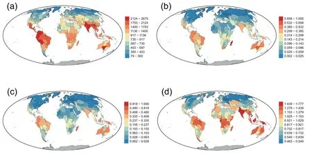
Fig.1.Geographic patterns of (a) genus richness,(b) taxonomic endemism (TE),(c) phylogenetic endemism (PE),and (d) relative phylogenetic endemism (RPE) for genus-level angiosperm assemblages across the world.TE and PE were scaled to vary between zero and one.

Given the expected correlations between richness and endemism based on the null hypothesis,it is important to also examine significant departures from the randomized expectation.Areas of significantly high TE are shown in Fig.2,along with differences in significance in PE (areas of significantly high PE are shown in Fig.3).

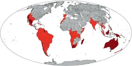
Fig.2.Differences between significance patterns of phylogenetic endemism(PE)and taxonomic endemism(TE).Dark red:significantly high in both PE and TE(N=23);bright red:significantly high only in PE (N=66);tan: significantly high only in TE (N=3).

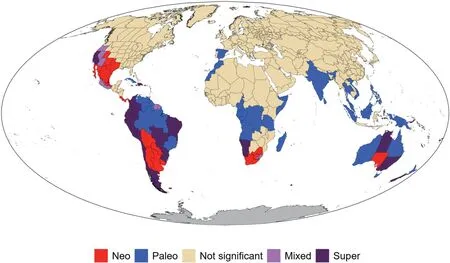
Fig.3.Global patterns of genus-level angiosperm endemism identified by categorical analyses of neo-and paleo-endemism(CANAPE),a phylogenetic approach identifying centers of phylogenetic endemism.The red color indicates centers of neo-endemism;the blue color indicates centers of paleo-endemism;the two purple colors indicate centers with a mixture of neo-endemism and paleo-endemism,with the darker purple color further indicating centers of super-endemism.

The result of the CANAPE analysis(Fig.3)showed that 89(23%)of the 391 regions analyzed in this study were significant centers of PE for angiosperm genera,of which 30,24,10 and 25 regions were determined as centers of paleo-endemism,neo-endemism,mixedendemism,and super-endemism,respectively.The vast majority of centers of PE were located in the tropics or Southern Hemisphere(Fig.3).Furthermore,all regions of South America and Australia were centers of PE,nearly all of which belonged to three of the four CANAPE types (paleo-endemism,neo-endemism,and superendemism).In Africa,centers of PE occupied about one third of the continent,the vast majority were located in the southern part of Africa,and most were centers of paleo-endemism.In North America,all centers of PE were located in the western and southwestern parts of the continent,and none of them were centers of paleo-endemism.In contrast,the vast majority of the regions in India and South Asia were centers of paleo-endemism (Fig.3).

3.2.Geographic,climatic,and historical correlates of endemism

For a given endemism metric,the direction and strength of the relationships between the metric and a geographic or climatic variable,across the 12 geographic and climatic variables examined in this study,were similar in correlation coefficients and standardized coefficients of regression (Figs.4 and S2).Similarly,for either statistical coefficient,patterns in direction and strength of the relationships between an endemism metric and a geographic or climatic variable across the 12 variables were similar among TE,PE and RPE (Fig.S2).Consequently,our summary of the relationships between endemism metrics and geographic or climatic variables focuses on TE and PE based on correlation coefficient in bivariate analysis,and reports the results of variation partitioning analyses for TE in the supporting information(Figs.S3 and S4).

Of the two geographic variables,elevational range was correlated with PE more strongly than was sampling area(r=0.433 and 0.247).For the six variables representing current climatic conditions,the three temperature-related variables were more strongly correlated with PE than were the three precipitation-related variables (Fig.4),with mean annual temperature having the strongest relationship with PE(r=0.758),which was followed by minimum temperature of the coldest month (r=0.704).The four historical climatic variables were negatively correlated with PE,with temperature anomaly having the strongest relationship with PE(r=-0.504;Fig.4).

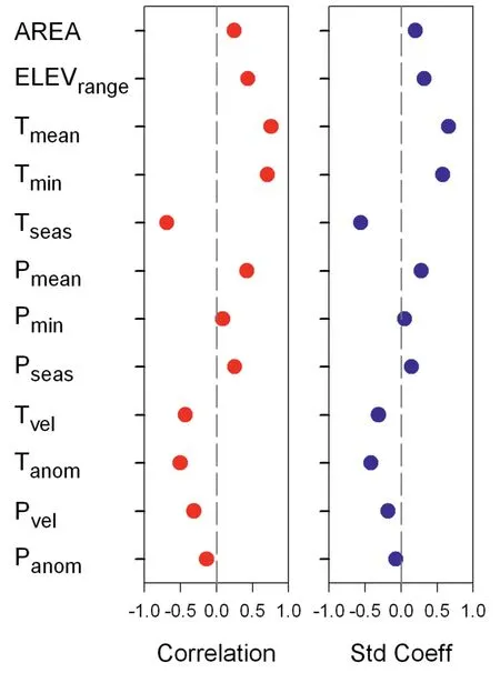
Fig.4.Pearson's correlation coefficient(red)and standardized coefficient of regression(blue) between phylogenetic endemism (PE) and each of geographic,climatic and historical climatic variables.Abbreviations for geographic variables are:AREA=area of geographic region,ELEVrange=elevational range;abbreviations for current climatic variables are:Tmean=mean annual temperature,Tmin=minimum temperature of the coldest month,Tseas=temperature seasonality,Pmean=annual precipitation,Pmin=precipitation during the driest month,Pseas=precipitation seasonality;abbreviations for historical climatic variables are: Tanom=temperature anomaly,Panom=precipitation anomaly,Tvel=temperature velocity,Pvel=precipitation velocity.

Among the three pairwise combinations of the three sets of explanatory variables,the combination of current climatic variables and geographic variables explained the largest amounts of the variation in PE (80.3%),nearly all of which were independently explained either by current climatic variables or by geographic variables,with the former explaining more than twice as much variation in PE as the latter (Fig.5).Current climatic variables and historical climatic variables together explained 64.6% of the variation in PE,of which more than half was independently explained by the former (Fig.5),and a small portion was independently explained by the latter.Geographic variables and historical climatic variables together explained only 36% of the variation in PE,and differences among the three portions of the explained variance(i.e.,explained independently by either set of variables and jointly by the two sets) were relatively small (Fig.5).

Fig.5.Partition of the variation in genus-level phylogenetic endemism of regional angiosperm floras across the world explained by current climatic variables(C),historical climatic variables(H),and geographic variables (G).Each variation partitioning analysis included two sets of explanatory variables.Geographic variables include area of geographic region,and elevational range;current climatic variables include mean annual temperature,minimum temperature of the coldest month,temperature seasonality,annual precipitation,precipitation during the driest month,and precipitation seasonality;historical climatic variables include temperature anomaly,precipitation anomaly,temperature velocity,and precipitation velocity.

When all the three sets of the explanatory variables were considered,81.4% of the variation in PE was explained by the variables,more than half of which was independently explained by current climatic variables (Fig.6).The set of geographic variables and the set of historical climatic variables independently explained 15%and 1%of the variations in PE,respectively.The variation in PE that was jointly explained by two or three sets of the variables was less than 15% (Fig.6).

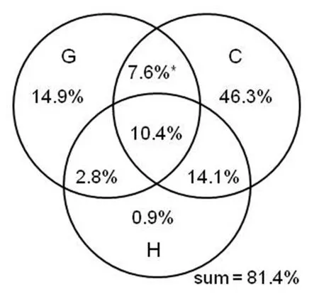
Fig.6.Pure and shared effects of three sets of explanatory variables on genus-level phylogenetic endemism of regional angiosperm floras across the world.Abbreviations of the three sets of explanatory variables: G=geographic variables,C=current climatic variables,H=historical climatic variables.See the Materials and Methods for details about the three sets of explanatory variables.Asterisks indicate negative values resulting from variation partitioning analysis.

The results from ANOVA comparing the three types of phylogenetic endemism centers for individual climate variables showed that of the six current climatic variables,mean annual temperature and precipitation during the driest month showed a significant difference among the types of endemism centers (P<0.05) and annual precipitation showed a marginally significant difference(P=0.06;Table S1).When the four historical climatic variables were considered,three showed a significant difference among the types of endemism centers (P<0.05) and the other (i.e.,precipitation anomaly) showed a marginally significant difference(P=0.07;Table S1).When the ten climatic variables were considered collectively,nine differed significantly (P<0.05) or marginally significantly (P<0.10) between neo-and paleoendemism centers,and seven differed significantly or marginally significantly between mixed-and paleo-endemism centers;in contrast,only two differed significantly or marginally significantly between neo-and mixed-endemism centers(Table S1).

Regions belonging to the three types of PE overlapped to a large degree in the ordination of the two first principal components of either current or historical climatic variables(Fig.7;Tables S2 and S3).Discriminant function analysis (Fig.S5) also showed considerable overlap among the three types;however,multivariate analysis of variance (MANOVA) showed a statistically significant difference among the centroids of the three types for both current and historical climatic variables (Table S4),indicating that despite the overlap among them,the types are different when all variables are combined.

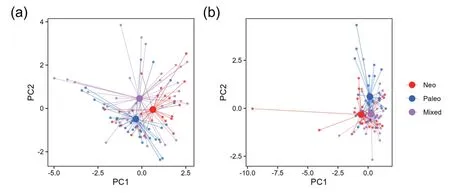
Fig.7.Ordination of phylogenetic endemism centers of angiosperm genera based on the first two principal components of the six current climatic variables (a),and the first two principal components of the four historical climatic variables (b).PC1 and PC2 in panel a explained 46.5% and 27.0% of the variation in the current climatic variables,and PC1 and PC2 in panel b explained 46.2%and 30.8%of the variation in the historical climatic variables.Details about the two principal component analyses were reported in Tables S2 and S3.

4.Discussion

Our study showed that both taxonomic endemism (TE) and phylogenetic endemism (PE) are highest in tropical regions with warm and humid climates,and tend to decrease with increasing latitude(Fig.1).However,there was a notable asymmetry between the Northern and Southern Hemispheres,with the latitudinal decrease being more marked in the Northern Hemisphere than in the Southern Hemisphere.These patterns of endemism for angiosperm genera are similar in many respects to those for mammals,trees,and seed plants (Rosauer and Jetz,2015;Sandel et al.,2020;Cai et al.,2023).The strong decline in endemism towards high latitudes in the Northern Hemisphere reflects,at least in part,the increase of land area,and thus larger potential taxon range size with increasing latitude(Orme et al.,2006;Sandel et al.,2020;Guo et al.,2022).In contrast,land area in the Southern Hemisphere declines towards high latitude,tending to produce smaller ranges(Orme et al.,2006) and higher endemism (Sandel et al.,2020) at higher latitudes.

Our study showed that raw PE is strongly correlated with raw TE in regional floras of angiosperms.However,our study also showed that regions with relatively low TE may have significantly high PE(Fig.2),indicating that it is necessary to consider the significance of both TE and PE when assessing endemism of a region.Furthermore,PE-based approaches allow one to distinguish between centers of paleo-endemism and those of neo-endemism.

Patterns of PE are ultimately driven by some combination of TE and phylogenetic uniqueness (i.e.,dissimilarity in evolutionary history between lineages inhabiting an area) (Sandel et al.,2020).The latter appears to dominate our results,since only 26 areas are significantly high in TE but 89 are significantly high in PE! Thus when one adds a phylogenetic component via CANAPE one uncovers much more endemism that is due to the way the cooccurring lineages are related to each other.For example,there are three areas that are significantly high in TE but not PE;in this case the rare genera there must be randomly scattered across the phylogeny.When the rare genera in an area are related,because of the shared deeper branches that are also range-restricted,this can result in a region being significantly high in PE but not TE.

We found that endemism of angiosperms is higher in regions with greater area and elevational range.On the one hand,regions with larger areas and elevational ranges tend to have higher topographical heterogeneity,which would lead to higher diversity of small habitats supporting more small-ranged species(McFadden et al.,2019).On the other hand,higher topographic heterogeneity often creates more dispersal barriers that may lead to higher speciation rates (Quintero and Jetz,2018),creating more smallranged genera and thus higher endemism.Our finding is consistent with the suggestion made in previous studies that topographic heterogeneity promotes endemism (Sandel et al.,2020).

Of the six current climatic variables examined in this study,the three temperature-related variables were more strongly associated with endemism metrics,compared to the three precipitationrelated variables,with mean annual temperature,temperature of the coldest month,and temperature seasonality all being strongly correlated with PE(positively for the former two and negatively in the latter).Annual precipitation was moderately and positively correlated with PE.On the one hand,warm and humid climates tend to have high energy availability,which would increase the opportunity for evolving new lineages,which would in turn promote endemism (Jetz et al.,2004).On the other hand,for a given size of area,warmer and more humid climates are expected to support larger sizes of populations,which would favor rangerestricted lineages (Jetz et al.,2004;Ricklefs,2010).Our study found that regions with high temperature seasonality support low endemism.This finding is consistent with the Rapoport's rule(i.e.,higher climatic seasonality selects for lineages having larger geographic ranges and broader climatic tolerances;Stevens,1989)and with previous findings for vertebrates(Sandel et al.,2011).It is likely that mean annual temperature and temperature seasonality are primary drivers of the latitudinal gradient of angiosperm genus endemism,particularly in the Northern Hemisphere.

High climatic anomalies and velocities during the Quaternary glacial-interglacial oscillations are likely to be associated with high species extinctions(Sandel et al.,2011),which is expected to cause low neo-endemism on the one hand and to increase paleoendemism on the other hand.Our study indeed showed that the four historical climatic variables each have a negative effect on endemism,i.e.,more unstable climates (higher velocities and anomalies) harbor less endemism,albeit that the effects are moderate or weak.The negative relationships between endemism and historical variables reflecting climate change that were revealed in this study for angiosperms are consistent to those observed in previous studies for vertebrates (Sandel et al.,2011).Our study found that temperature velocity and anomaly have a stronger effect on endemism than do precipitation velocity and anomaly.Regions with lower climatic velocity and anomaly would have higher climatic stability during cycles of glaciations,which would have allowed for the evolution of lineages with narrow physiological tolerances on the one hand,and reduced extinction risk of smallranged lineages on the other hand.Thus,climatically stable regions may act as refugia for endemic taxa during periods of climate changes(Dynesius and Jansson,2000;Jansson,2003;Sandel et al.,2011;Kissling et al.,2012;Thornhill et al.,2017;Enquist et al.,2019).Climatic velocity,which captures the important buffering effect of topographic heterogeneity on climate change (Scherrer and K¨orner,2011),is thought to be biologically more relevant in tracking migration of species during climate change,compared to climatic anomalies (Sandel et al.,2011).Our study showed mixed results on whether climatic velocities have a stronger effect on endemism than do climatic anomalies:precipitation velocity has a stronger effect than precipitation anomaly whereas temperature velocity has a weaker effect than temperature anomaly.

The three sets of explanatory variables(i.e.,geographic,current climatic,and historic climatic variables) together explained over three quarters of the variation in endemism,more than half of which was independently explained by current climatic variables.In contrast,historic climatic variables independently explained only about one percent of the variation in endemism.Thus,our findings suggest that climate changes during the Quaternary glacial-interglacial oscillations had a much weaker effect on global patterns of endemism of angiosperm genera,compared to current climate.This conclusion on patterns of angiosperm endemism is consistent with those on angiosperm species richness (e.g.,Qian et al.,2019).However,current and historical climatic variables jointly explained about a quarter of the variation in endemism,indicating that past climate change and current climate act together to determine global patterns of angiosperm endemism to a marked degree,as in global patterns of vertebrate endemism(Sandel et al.,2011).

Our study identified 89 regions as phylogenetic endemism centers,of which 30 are paleo-endemism centers,24 are neoendemism centers,and the others are mixed.Nearly all the endemism centers are located in tropical and subtropical regions,or in the Southern Hemisphere (Fig.3).Paleo-endemism centers are mainly located in Amazonia and Venezuela in South America,southern Africa (including Madagascar),and across a large geographic extent from India through Indochina to Australia and New Zealand (Fig.3).Most of the paleo-endemism centers are characterized by tropical moist forests.Paleo-endemism centers contain lineages that may have once been more widely distributed but now have restricted distributions,and thus have rare long branches in the phylogeny (Mishler et al.,2014).Thus,a center of phylogenetic paleo-endemism may indicate a long-term refugium.Neo-endemism centers are primarily located in western and southwestern North America,southern South America,southernmost Africa,and southern Australia(Fig.3).Neo-endemism centers contain areas with an over-representation of rare short branches.These areas may be places of recent divergence of lineages(Mishler et al.,2014).Since this study was done at the genus level,some neoendemism at the species level within otherwise widespread genera was likely missed,while paleo-endemism is likely well represented.

Significant centers of high PE found here using CANAPE were very similar to those found in Cai et al.(2023),with the exception of the Middle East and Japan (which were significant in their study but not ours),as well as South America and Australia (all of which was significant in our study but only parts of which were significant in theirs).However,the CANAPE classification was different in more cases.For example,Peru was identified as a center of mixed endemism in our study(Fig.3) but as a center of paleo-endemism in their study,while California was identified as a center of superendemism in our study but as a center of neo-endemism in their study(fig.3 in Cai et al.,2023).Note that the two studies differ both in their taxonomic scale (i.e.,genus in our study versus species in theirs)and also in taxonomic scope(angiosperms only in our study versus angiosperms plus gymnosperms in theirs),thus one must be cautious when comparing the results.Differences in identified centers of endemism between the two studies might reflect either the different phylogenetic scope (angiosperms vs.seed plants) or the different taxonomic rank of operational taxonomic units(genera vs.species),as noted above.Future studies are needed to further investigate these scaling issues.

The vast majority of the 36 biodiversity hotspots that have already been identified based on species richness and endemism(https://www.cepf.net/node/1996;Myers et al.,2000;Fu et al.,2022) are located in the centers of phylogenetic endemism identified in this study.However,a number of large regions that have been identified as the centers of phylogenetic endemism in this study do not have any previously identified biodiversity hotspots,indicating that some important biodiversity hotspots have been missed in previous richness-based selection of global biodiversity hotspots.Regions with the centers of phylogenetic paleoendemism that are not included in previous biodiversity hotspots include a combination of Amazonia and Venezuela in South America and a combination of several regions in West-Central Tropical Africa.Future selections of biodiversity hotspots should pay attention to these regions.Our study reveals some regions with low taxonomic endemism have high phylogenetic endemism,and these regions should also be considered when selecting additional biodiversity hotspots in future.Thus,our findings have important implications for biological conservation.

Author contributions

H.Q.conceived the study,prepared the data,conducted data analysis,and wrote most of the article;B.D.M.conducted data analysis and wrote part of the article;J.Z.prepared the data,and conducted data analysis;S.Q.conducted data analysis,and generated maps;all authors contributed to revisions.

Data accessibility statement

Plant distribution data are available in World Plants (WP;https://www.worldplants.de) and Plants of the World Online(POWO;http://www.plantsoftheworldonline.org).Current climate data are available at the CHELSA climate database (https://chelsaclimate.org/bioclim).Data of historical climate change are available at https://datadryad.org/stash/dataset/doi:10.5061/dryad.b13j1.

Declaration of competing interest

The authors have no competing interest to declare.

Acknowledgements

We thank anonymous reviewers for their helpful comments.

Appendix A.Supplementary data

Supplementary data to this article can be found online at https://doi.org/10.1016/j.pld.2023.11.004.