Efficient method to calculate the eigenvalues of the Zakharov–Shabat system

Shikun Cui(崔世坤) and Zhen Wang(王振)

1School of Mathematical Sciences,Dalian University of Technology,Dalian 116024,China

2School of Mathematical Sciences,Beihang University,Beijing 100191,China

Keywords: Zakharov–Shabat system,eigenvalue,numerical method,Chebyshev polynomials

1.Introduction

The nonlinear Schr¨odinger (NLS) equation is an important integrable equation that is derived from hydrodynamics and has been used to describe the propagation of optical solitons,Langmuir waves in plasma physics,Bose–Einstein condensation, and other physical phenomena.[1–4]Considering the initial value problem for the nonlinear Schr¨odinger(NLS)equation

whereq0(x) is a given function defined in Schwartz spaceS(R),subscriptsxandtrepresent the partial derivatives with respect to space and time, respectively.Whenλ=1, equation(1)is called a focusing NLS equation,and whenλ=−1,equation (1) is called a defocusing NLS equation.The NLS equation(1)is integrable and admits the following Lax pair:

whereψis a column vector with a shape of 2×1,kis a spectral parameter defined in complex field C,qis the potential function, and ¯qrepresents the complex conjugation ofq.A long but standard computation shows that the compatibility conditionψxt=ψtxfor the eigenfunctionψis equivalent to the NLS equation iqt+qxx+2λ|q|2q=0 for classical solutionsq.[6]Equation(2)is called the Zakharov–Shabat(ZS)system,which is thex-part of the Lax pair.The properties of the solution for the NLS equation are determined by the eigenvalues for the ZS system.[6]

The inverse scattering transform is an important method for solving integrable equations[5]and was a milestone of mathematical physics in the twentieth century.The inverse scattering transform of the NLS equation was proposed by Zakharov and Shabat.[6]The inverse scattering transform consists of direct scattering and inverse scattering.In direct scattering,we need to solve the ZS system and calculate the scattering data.The ZS system (2) is an eigenvalue problem and we need to find thekso that the ZS system exists as a nontrivial solution,wherekrepresents the eigenvalue andψis the corresponding eigenfunction.The eigenvalues for the ZS system consist of the discrete eigenvaluesκj, ¯κj(j=1,2,...,n1)and the continuous eigenvalues, whereκj ∈CR.The continuous spectrum of the ZS system is the real axis R, so we only need to calculate the discrete eigenvalues of the ZS system.The number of solitons that emerged inq(x,0) for the NLS equation is equal ton1.It is worth noting that the discrete eigenvalue of the ZS system can be an empty set and the solution will not evolve into solitons at this time.The amplitude of the soliton is determined by the imaginary part ofκj.The velocity of the soliton is determined by the real part ofκj.

It is important to develop simple and effective methods to calculate the eigenvalues of the ZS system.In most cases,the eigenvalues of the ZS system (2) cannot be obtained analytically.Therefore, it is difficult to calculate the eigenvalues of the ZS system analytically.Calculating the eigenvalues of the ZS system is an important step in the inverse scattering transform.If we cannot efficiently calculate the discrete eigenvalues of the ZS system,then we will not be able to solve the equation by the inverse scattering transform.Meanwhile,calculating the eigenvalues of the ZS equation is of great significance for the study of the evolution of solutions.By analyzing the number and magnitude of discrete eigenvalues,we can obtain the number and properties of solitons, which are closely related to the “soliton resolution conjecture”.[7]The numerical implementation of the inverse scattering transform attracted special attention when the NLS equation soliton solutions were proposed as potential candidates for fiber optical transmission.At present, increasing the accuracy and efficiency of computational methods for solving the direct ZS system remains an urgent problem in nonlinear optics.

Several numerical methods have been proposed to calculate the eigenvalues of the ZS system.Boffetta and Osborne developed a numerical algorithm for computing the direct scattering transform for the NLS equation.[8]Bronski considered the semi-classical limit of the ZS eigenvalue problem.[9]The finite difference method was used to compute the ZS eigenvalue problem numerically.[10,12]Hill’s method can be used to calculate the eigenvalues of the ZS system.[11]The Fourier collocation method (FCM) is an effective method to calculate the eigenvalues of the ZS system.[19]Vasylchenkovaet al.summarized several nonlinear Fourier transform(NFT)methods, and compared their quality and performance.[13]These methods can be divided into two types: the first is the iterative method for the zero point of Jost function,and the second is to solve the matrix eigenvalue problem.[14]

In this paper,we proposed an efficient numerical method for calculating the eigenvalues for the ZS system.We use Chebyshev polynomials and tanh(ax) mapping to extract the key information of the potential function, and then transform the ZS eigenvalue problem into a matrix eigenvalue problem.By solving the matrix eigenvalue problem, we can get the eigenvalues for the ZS system.This method not only has good convergence for the Satsuma–Yajima potential but also converges quickly for complex Y-shape potential.In addition,this method can be further extended to other linear systems.

This paper is structured as follows.In Section 2,the theoretical knowledge of Chebyshev polynomials is presented and our numerical method is presented in detail.In Section 3,our method is used to calculate the eigenvalues of the ZS system with the Satsuma–Yajima potential,the sech(2∈x)eisech(2∈x)/∈potential, and the exp(−ix)sech(x) potential.The convergence of our method is analyzed.Our method has spectral accuracy and its convergence rate is fast.Finally, some discussions are given in Section 4.

2.Methodology

The details of our method will be introduced in this section.Our method is summarized in the following steps.For the ZS system(2),Chebyshev polynomials are used to approximate the eigenfunctionψand the potential functionqwith the help of mappingH(x)=tanh(ax)(a ＞0).Using Chebyshev nodes,we turn the ZS eigenvalue problem into a matrix eigenvalue problem.We can then obtain the eigenvalues of the ZS system by calculating the matrix eigenvalue problem.

We define thenChebyshev nodes by

For the given functionf(x)defined in unit interval I,we can approximatef(x)by

where

Fis obtained by an appropriately scaled discrete cosine transform off(χ),F=[T(χ)]−1.

Tk(x)(k=0,1,...,n−1)is the Chebyshev polynomial of the first kind,

Chebyshev polynomials and their derivatives satisfy the relationship[15]

where

Using Eqs.(4) and (5), the function∂f/∂xcan be approximated by Chebyshev polynomials

For a given functiong(x)defined in real field R, we can approximateg(x) by Chebyshev polynomials and mappingH(x)=tanh(ax)

whereTR(x)=T(H(x))=[T0(H(x)),...,Tn−1(H(x))],H−1represent the inverse mapping ofH(x).H(x) is a one-to-one mapping, which maps the real field R to the unit interval I.The results of mappingH(x)are shown in Fig.1.

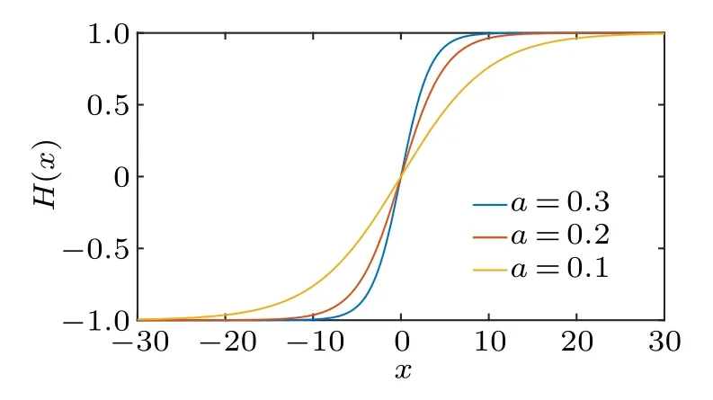
Fig.1.Results of mapping H(x)about different a.

By using Eqs.(5)and(7),and the chain rule,∂g/∂xcan be approximated by Chebyshev polynomials

In this way, the functiong(x) and its derivatives∂g/∂xare approximated by Chebyshev polynomials.

If a given function changes rapidly in a certain region,then we call this interval its‘rapid-changed interval.’H(x)=tanh(ax)changes near 0 rapidly,and its rapid-changed interval is expressed as[−L1,L1].L1is obtained by solving

wherea1is a real number close to 1.Takinga1=0.9951 as an example, the rapid-changed interval ofH(x)=tanh(0.3x) is[−10,10], the rapid-changed interval ofH(x)=tanh(0.2x)is[−15,15],and the rapid-changed interval ofH(x)=tanh(0.1x)is[−30,30].

The mappingH(x)distributes more Chebyshev nodes in the rapid-changed interval and distributes fewer Chebyshev nodes outside the rapid-changed interval.So in the rapidchanged interval,we can effectively identify the key information of the given function with the help of tanh(ax)mapping.

It is worth noting that the value ofawill influence the calculated result.Choosing an appropriateais important in our numerical method.For the selection of parametera(0＜a ＜1), we give the following recommendation.The value ofaaffects the range of rapid-changed interval and the range of rapid-changed interval will increase asadecreases.For the potential function defined in Schwartz space, it also has the rapid-changed interval.The rapid-changed interval of the potential function must be included in the rapid-changed interval of tanh(ax)mapping.If not,then we will be unable to completely extract the information of the potential function.

Rewriting the ZS system(λ=1)into a linear eigenvalue problem gives

Using Eqs.(7)and(8),we appropriate the eigenfunctionψ,ψxand the potential functionqby Chebyshev polynomials withnnodes,

wherej=1,2.

By substituting Eq.(10)into Eq.(9),we get

Settingx=H−1(χ),equation(11)is rewritten into

where

Equation(12)is recorded asAψ=ikψ,where

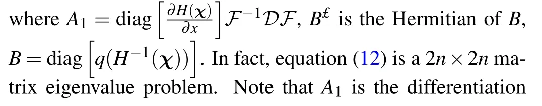
matrix for∂xin our method andBis a diagonal matrix that is composed of Chebyshev series forq(x).

The eigenvalue problem(12)can be solved by the quadrature right-triangle(QR)algorithm.[16]In the QR algorithm,the matrixAis decomposed intoA=QR,whereQis an orthogonal matrix andRis an upper triangular matrix.

The steps of theQRalgorithm are as follows:

diagonal elements ofAnare the eigenvalues ofAasn →∞.

Regarding the accuracy of this method, it does not need to truncate the interval and has spectral accuracy[19]for the smooth potential function.Because we do not truncate the calculated interval, our method will not produce a truncation error for the analytic potential.

3.Numerical results

Our method is used to calculate the eigenvalues of ZS system(λ=1)(2)with three potentials and the convergency of the method is analyzed.All of the numerical examples that are reported here are run on an Asustek computer with Intel(R)Core(TM)i7-11800H processor and 16 GB memory.

3.1.The Satsuma–Yajima potential

Our numerical method is used to calculate the eigenvalues of the ZS system(λ=1)with Satsuma–Yajima potential.Numerical results are compared with the analytical results and the performance of our numerical method is compared with the performance of the FCM.[19]

Whenq=Asech(x), Satsuma and Yajima exactly calculated the discrete eigenvalues of the ZS system.[17]Satsuma and Yajima found that the discrete eigenvalue in the upper-half complex plane C+is

wherenis a positive number satisfying.Due to the symmetry of the discrete eigenvalues,[17]the ZS system withAsech(x)potential has the discrete eigenvalues ¯κnin C−.

In the specific calculation, we calculate the eigenvalues ofq(x)=1.8sech(x).Whenq(x)=1.8sech(x),the ZS system has four discrete eigenvaluesκ1=1.3i,κ2=0.3i, ¯κ1=−1.3i and ¯κ2=−0.3i.The number of Chebyshev nodesnis set to 200 and the value ofais set to 0.15.The calculation results are shown in Fig.2.Figure 2(a) shows the calculated eigenvalues of the ZS system with the Satsuma–Yajima potential.There are four discrete eigenvalues in Fig.2(a),which is consistent with the theoretical result.Figure 2(b) shows the calculated eigenfunction in pointκ1and figure 2(c) gives the calculated eigenfunction in pointκ2.The absolute error between the calculatedκ1and the exactκ1is 1.85×10−15,and the absolute error between the calculatedκ2and the exactκ2is 1.61×10−16.The method takes about 0.2 s to finish.These results show that our method is efficient.

Fig.2.The calculated results of ZS system with 1.8sech(x) potential.(a) The calculated eigenvalues (red) and exact eigenvalues (blue) of 1.8sech(x)potential.(b)Numerical results of ψ1 (red line)and ψ2 (green line)at k=κ1.(c)Numerical results of ψ1 (red line)and ψ2 (green line)at k=κ2.

The stability and convergency of our method need to be analyzed.In area [a,n]∈[0.1,0.33]×[21,251], we calculate the eigenvalues of the ZS system withq(x)=1.8sech(x), the absolute error ink=κ1is shown in Fig.3(a).There are three routes in Fig.3(a)(blue route 1,black route 2,and green route 3),the convergency of our method is analyzed along the three routes.In the Fourier collocation method, the calculated interval is truncated to[−25,25].The relationship between the error andnis shown in Fig.3(b),the red line is the error curve calculated by the Fourier collocation method(FCM),the blue line is the error curve calculated by our method along Fig.3(a)“route 1”, the black line is the error bar calculated by our method along Fig.3(a) “route 2”, and the green line is the error bar calculated by our method along Fig.3(a) “route 3”.Figure 3(b) shows that our method is more accurate than the FCM and the convergence rate of our method is faster than FCM,so our method is more efficient.Because the error calculated by the FCM decays exponentially with the number of nodes,[19]the error of our method also decays exponentially with the number of nodes and its error decays faster than any power ofn−1.Thus the spectral accuracy of the method is confirmed.

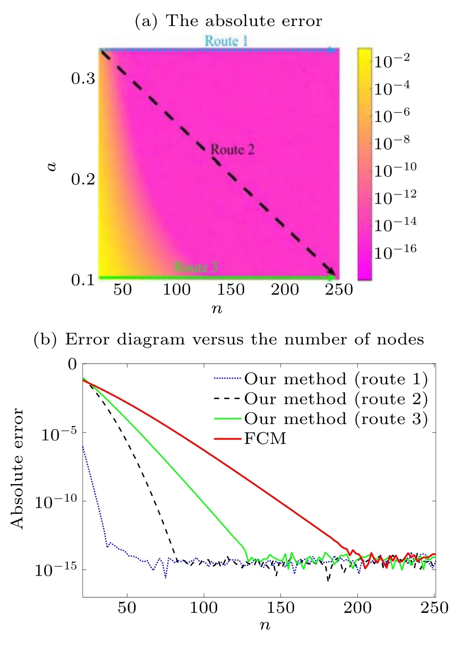
Fig.3.The absolute error in area[a,n]∈[0.1,0.33]×[21,251].(a)The absolute error picture(k=κ1).(b)The error diagram along route 1(blue line),the error diagram along route 2(black line),the error diagram along route 3 (green line), and the error diagram of the Fourier collocation method(red line).

We also explored the computational efficiency of our method and compared it with the FCM.We calculated the discrete eigenvalues of the 1.8sech(x)potential at different numbers of nodes and the time is shown in Table 1.

Table 1.The time required to complete the program at different nodes n.

The minimum error generated by our method is about 10−15level.This method can achieve machine accuracy.Since the calculated accuracy of the mathematical software is 16 significant figures, there will be an error of about 10−15level in the calculation process.Our method can greatly improve the calculated accuracy, especially when the number of Chebyshev nodes is small.

3.2.The Y-shape potential

Bronski computed the eigenvalues of the sech(2∈x)eisech(2∈x)/∈potential and found that the shape of the discrete eigenvalues is “Y”.[9]Settingn= 400 anda=0.02, our method is used to compute the eigenvalues of the sech(2∈x)eisech(2∈x)/∈potential with ∈=0.2,∈=0.1 and∈=0.05, and the calculated results are shown in Fig.4.The calculations are finished within 0.6 s.

When ∈= 0.2, there are three discrete eigenvalues in C+; when ∈=0.1, there are six discrete eigenvalues in C+;and when ∈=0.05, there are 12 discrete eigenvalues in C+.The calculated results are consistent with Bronski’s results(Ref.[9],p.385,Table 1).The calculated discrete eigenvalues become Y-shaped with the decrease of ∈,which are consistent with the theoretical results.

There are six discrete eigenvalues in C+in Fig.4(b),and their values are shown in Table 2.

Fig.4.The calculated eigenvalues of ZS system with sech(2∈x)eisech(2∈x)/∈potential(a=0.02).

From Table 2, we learn that the sech(0.2x)e10isech(0.2x)potential has two pure imaginary eigenvalues and four complex discrete eigenvalues in C+.Thus, theq(x,0) =sech(0.2x)e10isech(0.2x)initial profile will evolve into a secondorder breather and four solitons for the NLS equation.The Fourier spectral method[18]is used to calculate the evolution of the NLS equation withq(x,0)=sech(0.2x)e10isech(0.2x).The density of the calculated result is shown in Fig.5.In Figs.5(a)and 5(b), the initial profileq(x,0) = sech(0.2x)e10isech(0.2x)evolves into four solitons and a second-order breather, which is consist with Fig.4(b).

The correctness of the calculated result is verified by analyzing the convergence of the method.Whenn=400 anda=0.02, we obtain the eigenvalueκ1=−1.78524894765016×10−15+0.116148026898534i of the sech(0.2x)e10isech(0.2x)potential.Under differentnChebyshev nodes, we calculate the Cauchy error for theq(x,0)=sech(0.2x)e10isech(0.2x)potential atκ1.The calculated result is shown in Fig.6.The Cauchy error in Fig.6 is defined by

whereκ1(n)is the calculatedκ1undernChebyshev nodes andκ1=−1.78524894765016×10−15+0.116148026898534i.

Table 2.The values for the calculated discrete eigenvalues of the ZS system with sech(0.2x)e10isech(0.2x) potential.

Fig.5.The evolution of the initial profile q(x,0)=sech(0.2x)e10isech(0.2x)for the NLS equation.

Fig.6.The Cauchy error for the sech(2∈x)eisech(2∈x)/∈in κ1.

In Fig.6,the method gradually converges asnincreases,and generates an error of 10−15level.

3.3.The solitonic potential

Optical solitons have very important applications in all optical networks,optical communication,and optical logic devices.The soliton solution of the NLS equation is considered to be a potential solution for fiber optic transmission, so it is important to calculate its discrete eigenvalues.In this subsection, our method is used to calculate the eigenvalues ofqso=exp(−ix)sech(x).The initial value of the optical solitons can describe the propagation of signals in optical fibers.

As we all know,qsohas a discrete eigenvalueκ1=0.5+0.5i in C+.[10]Settingn=200 anda=0.1, our method is used to compute the spectrum ofqso=exp(−ix)sech(x), the calculated result is shown in Fig.7.The absolute error between the calculatedκ1and the exactκ1is 7.77×10−16,and the absolute error between the calculatedκ2and the actualκ2is 6.31×10−15.The calculation is finished within 0.3 s.Our method is more accurate and faster than the NFT method.[13]

Fig.7.The calculated eigenvalues of the qso=exp(−ix)sech(x)potential.

4.Conclusion

A numerical method is proposed to calculate the discrete eigenvalues for the ZS system.The tools that are used are Chebyshev polynomials and tanh(ax)mapping.We can effectively identify the key information of the given function with the help of tanh(ax) mapping and realize the high-efficiency calculation.

Our method has following advantages.First, we do not need to truncate the calculated region for analytical potentials,so our method will not produce truncation error when using Chebyshev polynomials to appropriate the given function.Second,the method can calculate the discrete eigenvalues for the ZS system with spectral accuracy.This method is highprecision and efficient.We calculate the discrete eigenvalues of the Satsuma–Yajima potential and compare the method with the Fourier collocation method,and find that the convergence rate of our method is faster than the Fourier collocation method.For the complex sech(2∈x)eisech(2∈x)/∈potential,our method still converges quickly.It is worth mentioning that our method can be further extended to solve other linear eigenvalue problems.

Acknowledgments

Project supported by the National Natural Science Foundation of China (Grant Nos.52171251, U2106225, and 52231011) and Dalian Science and Technology Innovation Fund(Grant No.2022JJ12GX036).