An Efficient Local Radial Basis Function Method for Image Segmentation Based on the Chan-Vese Model

Shupeng Qiu,Chujin Lin and Wei Zhao

School of Mathematics and Statistics,Guangdong University of Technology,Guangzhou,510520,China

ABSTRACT In this paper,we consider the Chan-Vese(C-V)model for image segmentation and obtain its numerical solution accurately and efficiently.For this purpose,we present a local radial basis function method based on a Gaussian kernel(GA-LRBF)for spatial discretization.Compared to the standard radial basis function method,this approach consumes less CPU time and maintains good stability because it uses only a small subset of points in the whole computational domain.Additionally,since the Gaussian function has the property of dimensional separation,the GA-LRBF method is suitable for dealing with isotropic images.Finally,a numerical scheme that couples GA-LRBF with the fourth-order Runge-Kutta method is applied to the C-V model,and a comparison of some numerical results demonstrates that this scheme achieves much more reliable image segmentation.

KEYWORDS Image segmentation;Chan-Vese model;local radial basis function method;Gaussian kernel;Runge-Kutta method

1 Introduction

Image segmentation is a challenging and complicated task in the field of image processing and has a wide range of applications in computer vision,such as medical image analysis,autonomous driving,remote sensing,security and protection monitoring[1-3].The major task of image segmentation is to divide a prescribed image into several nonoverlapping and disjoint regions according to characteristics such as color,gray level(intensity)and geometric shape.With the increasing demand for segmentation techniques,many methods have been proposed,including threshold-based methods,region-based methods,edge-based methods,PDE-based methods and emerging methods based on deep neural networks.Among these representative classes of methods,the latter two correspond to mainstream algorithms.Nevertheless,although deep learning methods such as fully convolutional networks perform well in terms of accuracy[4],they are not fully interpretable and require considerable time for neural network training.An image itself can be regarded as a discrete two-dimensional matrix,which can be modeled using continuous mathematical models based on partial differential equations(PDEs).Over the decades,PDE-based models have shown excellent applicability and efficiency due to their high mathematical significance.Among PDE-based models,active contour models are some of the most popular,including the parametric active contour model and the level set method.A parametric active contour model (Snakes) was first proposed by Kass et al.[5];however,in this model,the curves cannot enter deep areas of the image,and the initial curves must already be close to the edges of the image contours.To handle this limitation,the level set method was presented for flexibly handling topological changes in images [6-9].In this method,a contour curve is embedded into a higher-dimensional function,representing that the level sets of different topological structures in the evolutionary process all correspond to the same level.Therefore,such a level set function can automatically control topological changes.The Chan-Vese (C-V) model is a typical level set model using a variational principle [10],as an improved variant of the Mumford-Shah (M-S) model [11],in which the complex functional is simplified by assuming that the gray levels within homogeneous regions of an image are constant.Many works have proven that the C-V model can effectively improve the topological adaptation ability in curve evolution;therefore,it is a powerful tool for image segmentation and has attracted increasing attention from researchers[12-14].

Once the desired model has been derived,numerical simulation plays an important role in understanding the dynamic evolutionary process of active contours.At present,the finite differential method(FDM)has been widely applied to numerically solve the PDEs originating from the level set method in most cases;this method achieves reasonably satisfactory accuracy [11] but is computationally expensive.In addition,various traditional techniques and algorithms have been used to optimize the accuracy and results of image segmentation.Nonetheless,limited by the efficiency and data processing ability of these algorithms,many challenges still arise in practical applications.In recent years,the radial basis function (RBF) method has attracted much attention because of its simple format and high accuracy [15-19],and it has gradually developed into a significant numerical method in the scientific computing domain [20-23].However,for large-scale problems such as image processing,the RBF method incurs excessive computational costs due to the generation of a dense matrix[23-26],and the large condition number of this matrix can also causes calculation instability[27,28].To conquer this shortcoming,local RBF(LRBF)methods based on positive and conditionally positive global kernels have been developed,such as[29],which consider only the contributions from several neighboring points in the near field while ignoring the influence of distant points.The corresponding sparse interpolation matrix apparently reduces the condition number of the matrix,saves storage space and enhances computational efficiency.Other newly developed local methods,such as[30-32],can also be applied to achieve these benefits.

In this paper,based on a Gaussian (GA) kernel,a new LRBF scheme is developed for solving the C-V model accurately and efficiently.Specifically,since a high-dimensional exponential function can be separated along each dimension,the GA-RBF interpolation can be expressed in the form of a tensor product of multiple one-dimensional interpolations.This approach eliminates the isotropic property of radial basis functions;thus,it is suitable for treating inhomogeneous image problems,and afterward,a local scheme is obtained accordingly.

The remainder of this paper is organized as follows:Section 2 provides a brief review of the C-V segmentation model.Section 3 gives more details of the proposed LRBF method based on a Gaussian kernel and presents a fully discrete system obtained by combining the proposed method with the fourth-order Runge-Kutta method.Several numerical experiments are presented in Section 4 to verify the performance of the proposed method,including its accuracy,efficiency and stability.Finally,some conclusions and plans for further research are reported in Section 5.

2 Mathematical Model

In this section,we give a brief review of the C-V model,which is an active contour model for twophase segmentation based on the Mumford-Shah model.LetΩbe a bounded domain of R2,with the boundary∂Ω.LetIbe a given image,and letC(s)be a parameterized closed curve.Classical snakes and active contour models are designed to minimize the following energy functional:

whereL(C) is the length ofC;out(C) andin(C) represent the regions outside and inside ofC,respectively;c1andc2are two constants that denote the average intensities inside and outside ofC,respectively;andμ,λ1,andλ2are fixed nonnegative parameters.The first term controls the smoothness of the contour,while the latter two terms attract the contour toward objects in the image.

In problems of curve evolution,the level set method and,in particular,the ‘motion by mean curvature’approach of Osher et al.[6]have been used extensively.The curveCis implicitly represented via a Lipschitz functionφ,i.e.,C={(x,y)|φ(x,y)=0},and the evolution of the curve is given by the zero-level curve at timetof the functionφ(x,y,t),as shown in Fig.1.

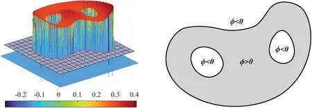
Figure 1:The level set function graph(left)and the zero-level curve graph(right)

With the introduction of the Heaviside functionHand the Dirac measureδ0,defined,respectively,as

the terms in the energy functional have the following forms:

Thus,the energyE(c1,c2,φ)can be written as

By keepingφfixed and minimizing the energyE(c1,c2,φ)with respect to the constantsc1andc2,it is easy to express these constants as functions ofφ,as follows:

For the corresponding“degenerate”cases,there are no constraints on the values ofc1andc2.Then,c1andc2are in fact given by[10]

By the calculus of variations,the Gateaux derivative of the functionalEcan be written as

Therefore,the functionφthat minimizes this functional satisfies the Euler-Lagrange equation=0.The steepest descent process for minimization of the functionalEcorresponds to the following gradient flow:

3 Numerical Method

3.1 The Global Radial Basis Function(GRBF)Method

In this section,we introduce the RBF method for the interpolation of scattered data.For a set ofNdistinct centers{x1,x2,...,xN}inΩ⊂Rn,an approximation(x)of a functionf(x)can be written in the form of a linear combination of radial basis functions(RBFs)as follows:

whereΦ(·)represents an RBF.Commonly used types of RBFs are listed in Table 1,in whichr=‖·‖is the Euclidean distance andc＞0 is the shape parameter.The coefficientsαjare obtained from the interpolation conditions at xi:

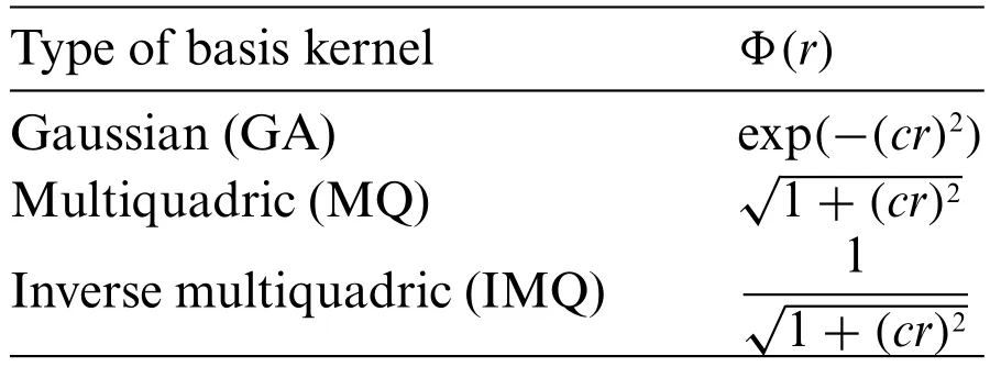
Table 1: Three common RBFs

Therefore,the following linear system of algebraic equations must be solved:

where A=[Φ(‖xi-xj‖)],i,j=1,2,...,N,α=[α1,α2,...,αN]T,and f=[f(x1),f(x2),...,f(xN)]T.After solving this system,the approximation off(x)and itsk-th order derivative can be obtained at any point inΩas

Because it always generates a dense interpolation matrix A,the standard RBF method is a global method that consumes more CPU time for larger-scale problems and can lead to unstable results because of ill-conditioned numbers.To handle these difficulties,we introduce the concept of local interpolation into the GRBF method.That is,for each evaluation point,we consider contributions only from its neighbors in the near field and ignore the effects from the far field.Because a sparse interpolation matrix is generated,this approach consumes less computing time.

3.2 Local Radial Basis Function Method Based on a GA Kernel(GA-LRBF)

For simplicity,we describe the method in two dimensions.ˆu(x,y) can be represented as an expansion of Gaussian radial basis functions:

whereΦjk(x,y)=exp(-c2((x-xj)2+(y-yk)2)).Since exponential functions have the property of separation,Eq.(15)can be written as

From the interpolation conditions on the data points(xm,yn)(m=1,2,...,Nx;n=1,2,...,Ny),we obtain the coefficient vector,and the approximation can be written as

whereΨj(x)andΨk(y)satisfy the interpolation conditions,i.e.,

To improve the stability of RBF interpolation,a localized approach was recently developed.The distinctive feature of this method is that only a few neighboring points are needed.Because it generates a sparse interpolation matrix,it consumes less computing time.Specifically,for points (xs,yl) (s=1,2,...,Nx;l=1,2,...,Ny),the local interpolation has the following form:

whereMsandMlare the numbers of closest points forxsandyl,respectively.SinceMs＜＜NxandMl＜＜Ny,all localMs×Mlmatrices can be extended to anNx×Nyglobal matrix by filling in zeros,and the obtained matrix is sparse.In particular,ifMs=Ml=3,the LRBF method becomes an FDM-type scheme,as shown in Fig.2,while ifMs=NxandMl=Ny,the LRBF method degenerates to the standard GRBF method.Compared with the GRBF method,this scheme consumes less CPU time because it yields a sparse interpolation matrix,and it maintains good stability because it uses only a small subset of points in the whole computational domain.Additionally,since the Gaussian kernel adopted as the RBF has the natural property of dimensional separation,the GA-LRBF method requires the storage of only a one-dimensional interpolation matrix and thus occupies less memory for numerical computation.Consequently,this method is suitable for dealing with isotropic images and efficient at manipulating massive-scale image information.However,different from[31,32],our proposed GA-LRBF method is essentially similar to the GRBF method but formally similar to the FDM;hence,the spatial derivative magnitude ofφis highly unlikely to be zero,meaning that this scheme can be freely applied.

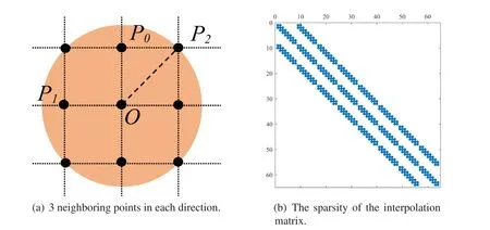
Figure 2:The GA-LRBF scheme with 3 neighboring points in each direction has a form similar to that of the FDM scheme.(a)3 neighboring points in each direction.(b)The sparsity of the corresponding interpolation matrix

To implement the GA-LRBF method for solving the C-V model,it is necessary to compute the differential operator

After the GA-LRBF method is applied to the C-V model,it can be expressed as a time-dependent semidiscrete nonlinear system

In this section,we consider the fourth-order Runge-Kutta scheme (RK4) for the C-V model.Lettingtn=nΔt(n=0,1,...,N) be uniform points in the time interval [0,T] with a time step ofΔt=T/N,we have

whereR(·)represents the right-hand side of the semidiscrete system.

4 Numerical Experiments

In this section,we report the numerical results obtained from the implementation of the proposed methods in Section 3.For this purpose,we present the following remarks:

· In this paper,all cases are calculated using a time step ofΔt=0.1 and a GA kernel with a shape parameter value ofc=1.How to choose the optimal shape parameter when using the meshless collocation method with the RBF approach is an open problem[27,28].Given that this is not the focus of our research,we have performed a simple numerical test using the GA-LRBF and GRBF methods with different shape parameter values.The numerical results indicate that the accuracy and efficiency of segmentation using the GA-LRBF method are relatively insensitive to the shape parameter value,but the same is not true for the GRBF method.Therefore,for better comparison in the numerical experiments,an appropriate shape parameter ofc=1 is consistently selected.· In practice,we use the regularized Heaviside functionHε(φ)in Eq.(8),defined as

and the corresponding regularized Dirac functionδε(φ)in Eq.(10)is given by

The parameterε=1 is selected in the following numerical experiments:

· To verify the influence of the initial contour on the subsequent evolution,we consider two types of initial level set functions.One is a circle contour,which is defined asφ0=r-whereciandcjdenote the half height and width,respectively,of the image andr=1/3ci.The other is a constant contour,which is defined asφ0=2 for the entire domain.

· To judge the effectiveness of image segmentation,we consider two classical evaluation indices defined as[33,34]

where “DICE”measures the spatial overlap between two target regionsAandBand “VOE”describes the error ratio of segmentation.For successful image segmentation,the values of“DICE”and“VOE”should tend toward 1 and 0,respectively.

Example 4.1.ThefirsttermoftheC-Vmodel,μ∇·(∇φ/|∇φ|),describesthesmoothnessofthe levelsetfunction.Totestitsinfluenceonevolution,wesolvetheC-Vmodelwithvariousvaluesofthe parameterμbyusingtheGA-LRBFmethodcombinedwithRK4.Theinitialcontouristakentobea circle.

Fig.3 displays the segmentation results for a 256 × 256 pixel image based on the C-V model withμ=100,100,10,1,0.1 and 0.It can be observed that smaller parameter values lead to better results;in particular,whenμis zero,there is almost no influence on evolution.The results are listed for comparison in Table 2.Moreover,during iteration,the divergence term imposes a heavy calculation burden.The same analysis is performed in the Appendix using the GRBF method,and we come to a similar conclusion.Consequently,to balance efficiency and accuracy,the parameterμis taken to be 0 in the following numerical examples.

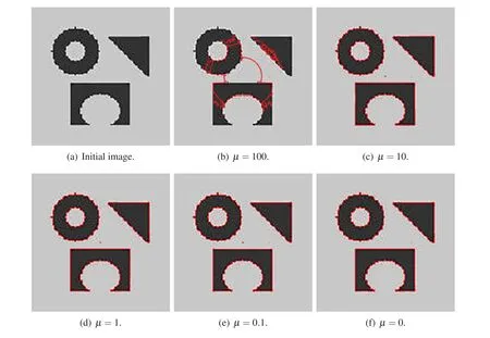
Figure 3:Evolution results for the initial image obtained using the GA-LRBF method combined with RK4 with different μ values

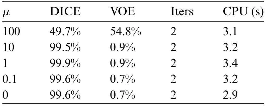
Table 2: Numerical results of using the GA-LRBF method combined RK4 with different μ values

Example 4.2.ThisexperimentisdesignedtotesttheperformanceoftheLRBFmethod.Forthis purpose,weapplytheLRBF,GRBFandFDMschemestodiscretizethespatialvariablesoftheC-V modelandtheRK4schemefortemporaldiscretization.Bothcircularandconstantinitialcontoursare considered.

Fig.4 shows the results of the three numerical methods for a 238×200 pixel image with parameters ofμ=0 andλ1=λ2=1.For a constant initial contourφ0=a(ais a constant),sinceμ=0,we note thata=1 should be avoided because it would cause the right-hand term in Eq.(10) to be 0,leading to stationary evolution.As shown in these figures,for a circular initial contour,the numerical results of all three methods converge to the image boundaries,whereas for a constant initial contourφ0=2,the FDM does not work,but the two RBF methods maintain good results.More results of these three methods are listed for comparison in Table 3.We conclude that the initial contour has a dramatic influence on the numerical results of the FDM but has little effect on the results of the two RBF methods.Thus,the RBF methods are effective computing tools for image segmentation;in particular,the LRBF method consumes less CPU time than the GRBF method.It is worth noting that the presented scheme is robust to and independent of the initialization,even without manual initialization;consequently,there is no need for complex and expensive reinitialization of the level set function to maintain numerical stability,which may be necessary in the traditional method[11].

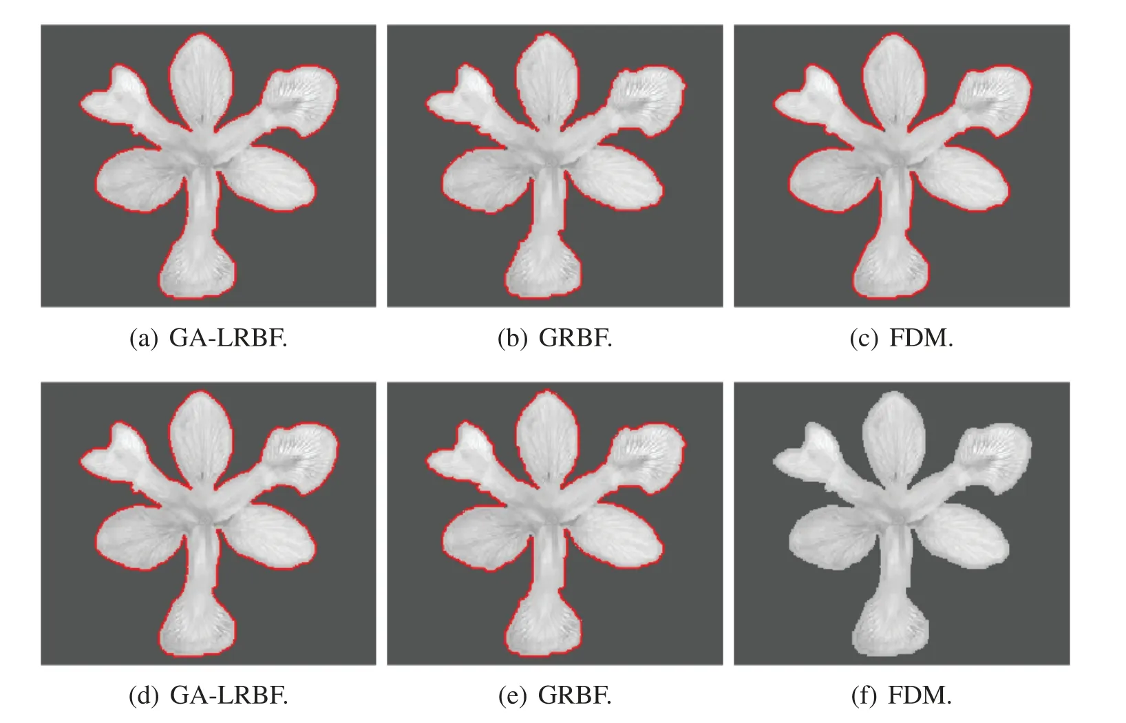
Figure 4: Evolution results of three numerical methods with (a-c) a circular initial contour and(d-f)a constant initial contour φ0=2

Table 3: Numerical results of these methods for two different initial contours

Example 4.3.ThisexperimentisdesignedtotesttheperformanceofRK4.WeapplytheGA-LRBF methodtodiscretizethespatialvariablesoftheC-Vmodel,andthecommonlyusedforwardEulerscheme isintroducedfornumericalcomparison.Twodifferentinitialcontours(circularandconstant)areused.

We select three initial images as shown in Fig.5.Table 4 lists numerical results of LRBF combined with RK4 and Forward Euler schemes for the edge segmentation problem.As expected,the convergence rate of the RK4 scheme is also much faster than that of the forward Euler scheme.Additionally,for clarity,Figs.6 and 7 display the contour evolution on these three images.As we can see that,for the edge segmentation problem(Fig.5a),the forward Euler method with a constant initial contour is less effective than this method with a circular initial contour.In particular,for images with holes(Figs.5b and 5c),the forward Euler method cannot effectively separate the image from the background regardless of whether a constant or circular initial contour is used.However,RK4 is minimally affected by the above problems.

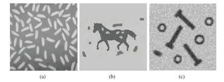
Figure 5:Three initial images,with pixel of(a)256×256,(b)256×256,and(c)160×160

Table 4:Numerical results obtained by the RK4 scheme and the forward Euler scheme for temporal discretization

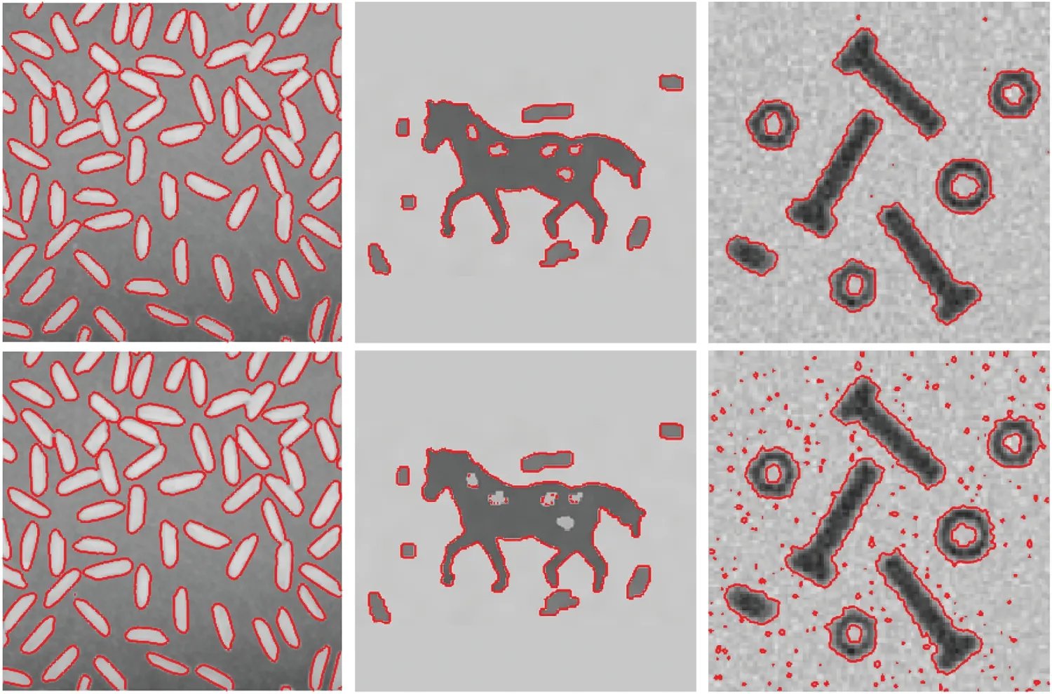
Figure 6:Evolution results obtained by RK4(first row)and the forward Euler scheme(second row)with a circular initial contour

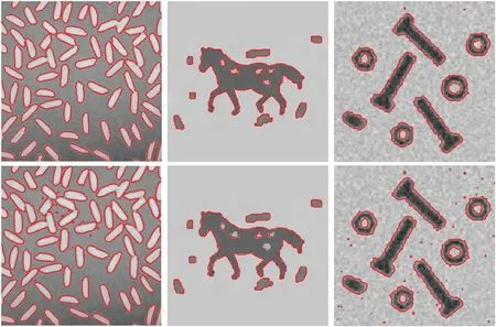
Figure 7:Evolution results obtained by RK4(first row)and the forward Euler scheme(second row)with a constant initial contour φ0=2

5 Conclusion

In this paper,we presented a novel numerical method to solve the C-V model arising in image segmentation,in which the GA-LRBF and RK4 schemes were used for spatial and temporal variables,respectively.The LRBF method achieved improved efficiency and stability compared with the standard GRBF method because it used only a few neighboring points rather than all points in the domain.Furthermore,since the extensional function can be separated along each direction,it is suitable for the treatment of inhomogeneous image problems.Numerical results verify that the GALRBF method combined with RK4 can guarantee successful segmentation results with both circular and constant initial contours and even for images with holes.Therefore,this method is a powerful numerical tool for image segmentation.At present,the number of neighboring points is fixed for the GA-LRBF method;the question of how to determine the optimal number of points will be a focus of our work in the near future.

Acknowledgement:Authors would like to thank Dr.Rui Zhan at Guangdong University of Technology for providing many valuable suggestions for this research.

Funding Statement:This work was sponsored by Guangdong Basic and Applied Basic Research Foundation under Grant No.2021A1515110680 and Guangzhou Basic and Applied Basic Research under Grant No.202102020340.

Author Contributions:Shupeng Qiu: Conceptualization,Methodology,Software,Investigation,Formal Analysis,Writing Original Draft;Chujin Lin:Visualization,Investigation;Wei Zhao:Conceptualization,Funding Acquisition,Resources,Supervision,Writing Review&Editing.

Availability of Data and Materials:The authors confirm that the data supporting the findings of this study are available within the article.

Conflicts of Interest:The authors declare that they have no conflicts of interest to report regarding the present study.

Appendix

Fig.8 displays the segmentation results for a 256×256 pixel image obtained using the GRBF method combined with RK4 withμ=100,100,10,1,0.1 and 0 based on the C-V model.It can be observed that smaller parameter values lead to better results;in particular,whenμis zero,there is almost no influence on evolution.The results are listed for comparison in Table 5.

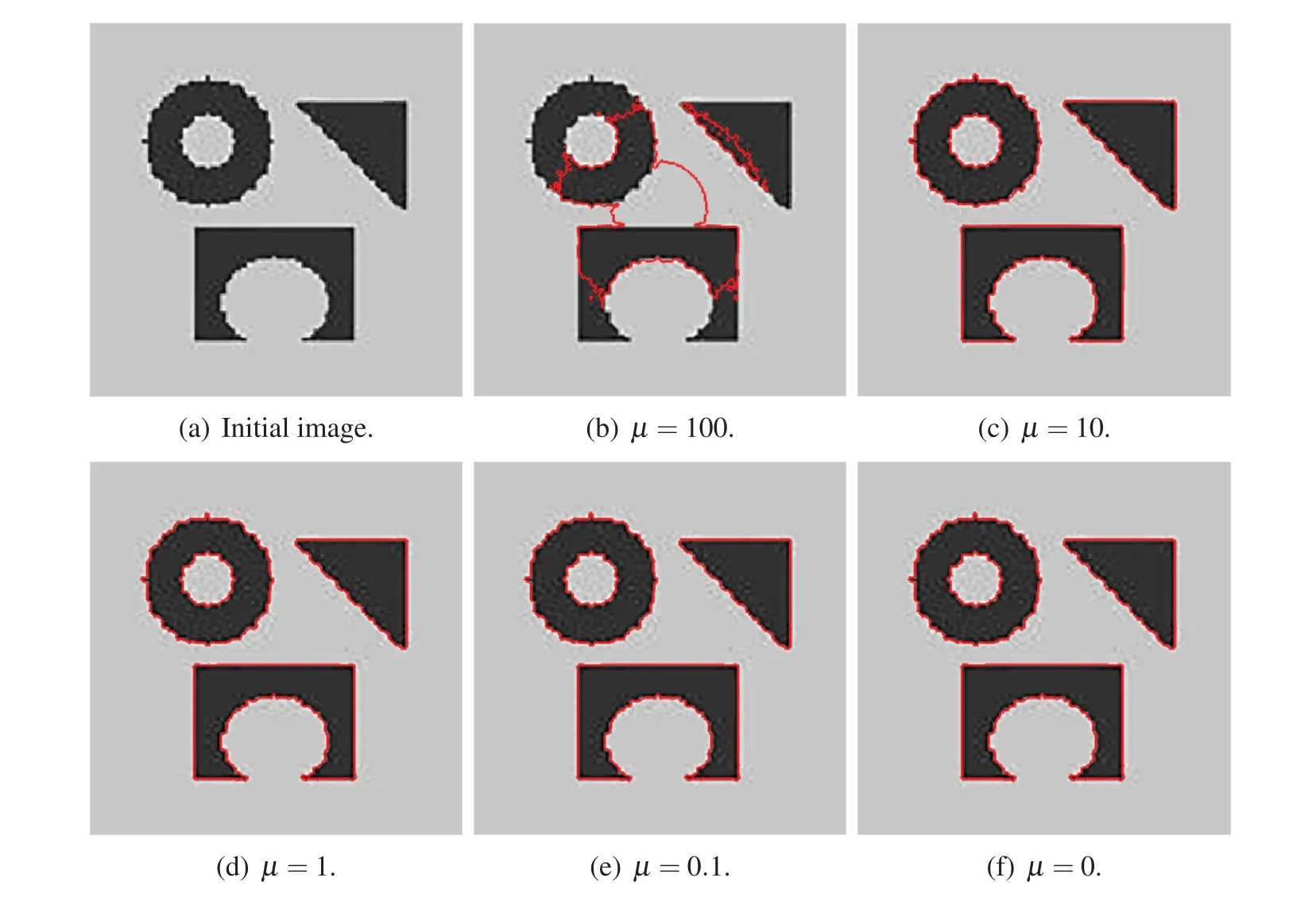
Figure 8:Evolution results for the initial image obtained using the GRBF method combined with RK4 with different μ values

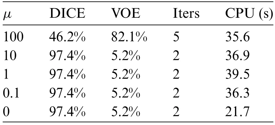
Table 5: Numerical results of using the GRBF method combined with RK4 with different μ values