A Metadata Reconstruction Algorithm Based on Heterogeneous Sensor Data for Marine Observations
GUO Shuai, SUN Meng, and MAO Xiaodong
A Metadata Reconstruction Algorithm Based on Heterogeneous Sensor Data for Marine Observations
GUO Shuai1), *, SUN Meng2), and MAO Xiaodong2)
1),,266520,2),,266520,
Vast amounts of heterogeneous data on marine observations have been accumulated due to the rapid development of oceanobservation technology. Several state-of-art methods are proposed to manage the emerging Internet of Things (IoT) sensor data. However, the use of an inefficient data management strategy during the data storage process can lead to missing metadata; thus, part of the sensor data cannot be indexed and utilized (., ‘data swamp’). Researchers have focused on optimizing storage procedures to prevent such disasters, but few have attempted to restore the missing metadata. In this study, we propose an AI-based algorithm to reconstruct the metadata of heterogeneous marine data in data swamps to solve the above problems. First, a MapReduce algorithm is proposed to preprocess raw marine data and extract its feature tensors in parallel. Second, load the feature tensors are loaded into a machine learning algorithm and clustering operation is implemented. The similarities between the incoming data and the trained clustering results in terms of clustering results are also calculated. Finally, metadata reconstruction is performed based on existing marine observation data processing results. The experiments are designed using existing datasets obtained from ocean observing systems, thus verifyingthe effectiveness of the algorithms. The results demonstrate the excellent performance of our proposed algorithm for the metadata reconstruction of heterogenous marine observation data.
Internet of Things (IoT); sensor data; data swamp; metadata reconstruction
1 Introduction
Marine environmental data represent a comprehensive concept, involving hydrology, meteorology, chemistry, bio- logy, geology, earth geography and other disciplines. Thesemainly include the atmosphere (., temperature, wind, rain, clouds, fog), hydrology (sea temperature, salinity, depth, tides, waves, currents,.), and various types of seabed to- pography, landform, geology, gravity, magnetism, seabed expansion data. With the rapid development of China’s marine observation technology, we have found more ways to use marine observation data (Xu., 2019). Recently, issues related to marine observation data have been recog- nized worldwide. In China, the marine information network constructed frommarine observation data plays a significant role in the country’s marine economy and security, marine science, and national defense. Undoubtedly, the processing of marine observation data is crucial in using these data. We can analyze plenty of serviceable information from it, which can be used in marine monitoring, data mining, informationtransmission, and feedback of results. As these marine observation data are obtained in various ways, the enormous amount of collected data may also varyin terms of quality and quantity. Such massive volumes of data can lead to an information explosion if not handled appropriately. McCrory (2010) proposed a novel concept called ‘data gravity’, wherein data, services and applications are treated as planets, each having its own gravity. From this data-centric perspective, where data on services and applications are captured because of their increased mass and density, it is fair to say that the processing of ma- rine observations has an essential function during the over- all ocean data observation process. However, most of the raw time series data (Bettini., 1998), including struc- tured data (relational database), semistructured data (XML and HTML files) and nonstructured data (pictures, videos,.), are stored isolated in different places. Thus, the mainchallenge is how to store and leverage those data efficiently in order to meet the huge demand for data analysis.
Numerous studies have provided a data storage framework for marine observation big data. Traditional data ware- houses have failed to satisfy the need for big data analysis due to the extract-transform-load (ETL) process (Vassiliadis., 2002). Accordingto IBM Research, nearly 70% of the time spent on analytic programs can be linked to data identification, purification and integration. During ETL, raw marine observation data will be preprocessed and defined in a fixed schema before storing them in a data warehouse a process that increases the cost (in terms of time and money) of data processing. Moreover, it destroys the essential characteristics of raw time series data by ex- tracting partial data and transforming them into different schemas.
The current purposes of marine big data analysis are to find regular patterns and obtain potential value from tremendous marine observation data without any forehead knowledge. As far as we know, traditional data warehouse objects for big data analysis are highly structured datasets with small sizes and predefined schema, which are not fle- xible and completely against the fundamental concept of big data analysis. An emerging concept called ‘data lake’ has been proposed to address all the challenges mentionedabove. It has also increasingly attracted more attention from data analysis experts. A data lake works well at storing marine observation big data in raw format (Alrehamy and Walker, 2015). It applies a distinct identifier and predefined metadata instead of the ETL process to manage all raw data. The flexible framework enables data scientists and average data consumers to query relevant data by le- veraging purpose-built schema. Furthermore, metadata ad- ministration acts as a central component of the data lake ar- chitecture. Generic metadata and corresponding maintenance mechanisms what prevent a data lake from becoming a data swamp (Terrizzano., 2015). Thus, many resear- chers are devoted to designing metadata management for data lakes. With the explosion of marine observation data and the increasing demand for data interconnection, it is unrealistic to assume that every piece of metadata is defined as well as it supposes should be. This leads us to a question, ‘How can we take efficient measures to restore a data swamp into a data lake?’ While other studies have primarily focused on different artificial intelligence applications implemented in data lakes, and those topics will continue to yield innovations, numerous metadata reconstruction problems must also be addressed so that data lakes can become more fully functional.
In the paper, we propose an automatic metadata reconstruction (AMR) algorithm to reconstruct metadata for marine observation in a data swamp (Qiu., 2016). The first obstacle to overcome in obtaining the characteris-tics of marine observation data is that we consider allmessages to be concealed. Through an analysis of the tem- poral series datasets, we can recognize what kinds of tasks they are, which field they most likely come from, and whatinformation about them is valuable. Finally, we reconstructour metadata based on the previous recognition results. Our principal achievements include the following:
We introduced the concept of data lake and revealed its advantages and disadvantages for marine observation time-series data storage by comparing it with the data warehouse. Thus, the data swamp problem is brought out.
We designed a MapReduce-based data preprocessor for dealing with data in data swamp. By leveraging the technology of data mining and machine learning, we are able to extract the characteristics of raw marine observation dataand denote them as input tensors of neural networks beforeimplementing clustering (Alex and Alessandro, 2014). We also discovered the emergentrelationship between the data obtained by the various methods and the results of the preprocessed data analysis, after which we transformed them into the corresponding geometrical patterns.
For agglomeration performance, we assessed the resemblance between the input raw time series data and the induced agglomeration performance. Eventually, we utilize identification results of marine observation tasks, fields, and sensors that obtain the marine data to reconstruct metadata (Xu, 2020).
We validated the usability of our algorithm by experimenting with ocean observation data (Jiang., 2021). The results indicate that our algorithm performs satisfactorily on metadata reconstruction for data swamp.
The remainder of this paper is structured as follows. Section 2 contains a description of data lake in detail with the main motivation of this paper. Our automatic metadata reconstruction AMR algorithm is discussed in Section 3. Section 4 explains the process of designing the experiments. This section also discusses how experiments on authentic datasets are performed to validate the effectiveness of our algorithm. Section 5 introduces some related works about data lakes and measurement coding with data swamps. Fi- nally, the paper is concluded in Section 6, in which the orientations for upcoming research are also given.
2 Background and Motivation
This section will elaborate on the concept of the data lake,enumerate several information technology (IT) enterprises (Google, Amazon,.) interested in data lake, discusses the advantages and disadvantages, and finally presents our motivation for this paper.
2.1 Data Lakes
James Dixon first proposed the idea of a ‘data lake’ on his blog in 2010. He argued that a traditional storage frame- work cannot satisfy the current need for marine observation big data. Thus, instead of using a data warehouse, a place filled with bottled waters displayed in a predefined schema, he wants to build a natural data lake where everyone can get water in their own ways. A data lake fulfills the requirements for fast data integration, while remainingthe characteristics and integrity of raw time series data. Nu- merous big tech enterprises have begun to build their own data lakes. For example, Google’s GooDs (Google Dataset Search) uses a post-analysis method to find the correlationby analyzing metadata (Halevy., 2016). Amazon applies the data lake concept to its Amazon Web Service (Jack- son., 2010). A data lake has its own advantages and disadvantages compared with a traditional data warehouse. More details are shown in Fig.1 and Table 1.
Advantages: Based on the Schema-on-read method, a datalake achieves fast data integration and skips the process ofraw data extraction, conversion, and cleansing. The costs of time and data processing are also reduced.
1) Quickly absorbs different types of data without chang- ing the current storage schema;
2) Low cost for data storage and processing;
3) Maintains the characteristics of raw data.
Disadvantages: Efficient method for metadata manage- ment is required. Otherwise, a data lake will eventually be- come a data swamp.
1) Quickly absorb different types of data without chang- ing the current storage schema;
2) Low efficiency under particular query;
3) Complicated approach for data management.
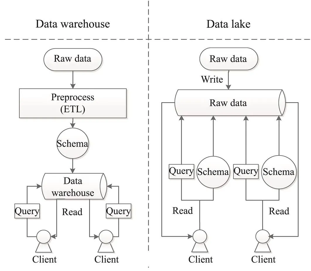
Fig.1 Comparison between the workflows of a data lake and a data warehouse.

Table 1 Comparison of a data lake versus a data warehouse
2.2 Motivation
Once a data lake is without its structure and governance, it becomes a data swamp (Hai., 2016). In such a scenario, data can no longer be found and queried owing to the absence of efficient procedures, criteria, and governance. With the rapid development of marine observation technology, data lakes have been fed with tremendous raw marine observation data.In recent years, many enterprises have begun to create their big data repositories by inputting everything into Hadoop, in which the computing and storage costs are acceptable (Golov and Ronnback, 2015). However, in most cases, only data providers are aware of the data they generate but fail to describe it as well-de- fined metadata, leading to situations wherein enterprises eventually lose control of the data in their data lakes. More- over, metadata management plays a vital role in operating data lakes; however, it becomes very challenging, time-con- suming, and expensive if the data lake is not maintained well (Satija., 2020; Sawadogo and Darmont, 2020). To summarize, dealing with data swamps is inevitable.
3 AMA Design
An AI-based metadata reconstruction (AMR) algorithm for data swamps is proposed in this section (O’Leary, 2014). Data fields and tasks are identified through the analysis of the raw collected data. An AMR architectural profile is illustrated in Fig.2. First, it preprocesses every loaded task data in the data lake. Next, the features of the preprocessed data are pulled by creating several approaches and then setting them into eigenvectors, which will be subsequently clustered by the machine learning algorithm. In the end, AMR automatically analyzes the raw collected data from the data swamp using the same process above. Then it calculates similarity to recognize the field and task and eventuallyreconstructs metadata.
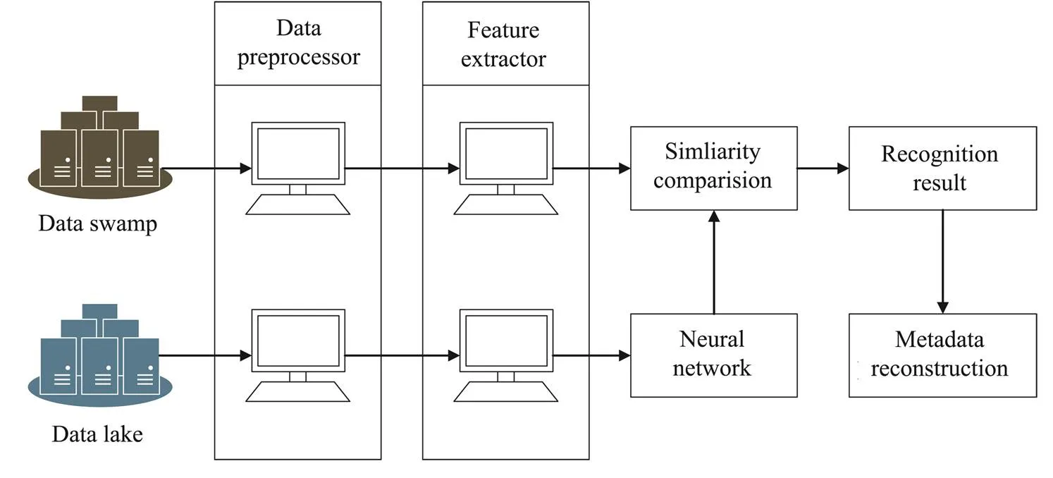
Fig.2 Architecture overview of the AMR.
3.1 Data Preprocessing
Here, we take as an example the observation of ocean data through Internet of Things (IoT) sensors (Atzori., 2010; Bandyopadhyay and Sen, 2011; Evans, 2011; Datta and Bonnet, 2015; Hu., 2020).A single ocean data observation task requires data to be acquired through different sensors in the IoT, each obtaining ocean data with its characteristics (Evans, 2011; Miorandi., 2012; Gubbi, 2013). Therefore, identifying the correlations between the data collected by various sensors by evaluating the raw values of the data obtained by the sensors is an extremely difficult task. AMR preprocesses the raw data based on a discretization approach and considers the sampling time; this contributes more to finding correlations from the data collected by each sensor from the ocean data observation task to which it belongs. First, a few defined notations are listed as follows:
represents the IoT field;represents an IoT marine observation task used in; For any task, we represent the set of all the sensors inby;represents IoT sensor data in; andr(=1, 2, ···,) represents sensor data of sensorS.
In addition,is denoted by a two-dimensional (2D) matrix, and we assumehassensors withtime slots de- noted as follows:

3.1.1 Discretization based on data value
We design a Map function to preprocessby leveraging the data normalization method (see detail in Algorithm 1). First, we definite a×matrix+and a thresholdare applied to discrete range (0, 1) intoparts. For eachin+:
Algorithm 1: Map function for data discretization based on data value
Input: IoTsensor data, threshold
1 min() ←( );
2 max() ←( );
3 tempKey=+'';
4 for=0 todo
5 clear tempValue;
6 for=0 todo
9 end
10 EmitIntermediate(tempKey, tempValue)
11 end
3.1.2 Discretization based on data offset
Next, we design another Map function to preprocessby leveraging the data normalization method (see detail in Algorithm 2). Here, we definite a (−1)×matrix+; furthermore, for eachin+, every entry represents the data offset between two neighboring time slots values.
Algorithm 2: Map function for data discretization based on the data offset
Input: IoTsensor data
1 tempKey=+'';
2 for=0 todo
3 for=0 todo
5 end
6 end
7 for=0 todo
8 clear tempValue;
9 for=0 todo
11 end
12 EmitIntermediate (tempKey, tempValue);
13 end
3.2 Feature Tensor Extraction
We propose two approaches called horizontal correlation extraction and vertical correlation extraction, respectively, to obtain optimal clustering results. These two approaches leverage the Markov transition probability matrix and statistical distribution as the feature tensor of IoT sensor data, respectively (Wu., 2014).
3.2.1 Vertical correlation extraction
We used the Markov model to accomplish feature tensor extraction and determine the vertical correlation in IoTsensor data. The next data state could be predicted in terms of the previous data state by calculating the transition probability matrix. AMR leverages the transition probability matrix as a feature matrix extracted from preprocessed data+, which hastime slots, and each time slot represents a stateψat that time. Each stateψconsists ofpreprocessed data fromsensors. Thus, we define+as shown in Eq. (2):

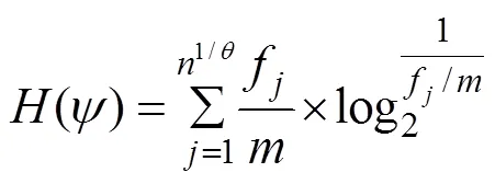
A thresholdis utilized to a discrete data value and thus determines the data state, loading into K-order Markov Chain. AMR chooses the optimalorder and thresholdin terms of conditional entropy result. More details are shown in Algorithm 3. The mathematical meaning of information entropy is to characterize the degree of stochasticity of a dataset, with increasing entropy indicating an increasing degree of stochasticity and decreasing entropy indicating a lower degree of stochasticity. The whole process involves five steps as follows:
Step 1.=+=(1,2, ···,ψ). The marginal entropy can explicitly be written as Eq. (3).
Step 2. Considering 1-order Markov,1={(1,2), (3,4), ···, (ψ−1,ψ)}, the joint entropy(1,) is defined as Eq. (4).

Step 3. Calculate conditional entropy(1,) as shown in Eq. (5).

Step 4. Based on Steps 1–3, keep calculating the conditional entropy of K-order Markov. Eventually, the conditional entropy with K-order Markov is written as Eq. (6) in the following:

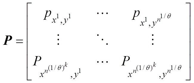
Step 5. For all the time slots in+, count the frequency ofψand denote it asf, where 1≤≤. Based on the conditional entropy result, AMR obtains a K-orders Markov Chain with thresholdand then calculates the transition probability matrix of each preprocessed set of data (see Eq. (7)) under different preprocess approaches:

Algorithm 3: Condition entropy calculation
Output: Conditional entropy
1+={1,2, ···,t}←
2 foreachÎtempKeydo
3 sort time slottby timestamp;
4t={0,1, ···,−1};
5 foreachÎtdo
6←total appearance times of;
7 end
8 for=0 to3−1 do
10 end
11 extend to 1-order Markov;
12t1={(0,1), (1,2), ···, (−2,−1)};
13 repeat steps 6–8;
16 end
18 extend steps 6–18 to K-order Markov;
20 end
21 return conditional entropy
3.2.2 Horizontal correlation extraction
We assume that the raw marine observation data from two different sensors during one task are related in order to determine the horizontal correlation in sensor data. By extracting the feature tensorof+, AMR utilizesas a characteristic to signify the entries in preprocessed data (You., 2005). The mathematical method we employed is the numerical distribution method. AMR obtains all the dual combinations for all the entries from each row of+and calculates their corresponding numerical distribution. Then, AMR goes through all the combinations and calculates the occurrence frequency of each scenario. Finally, AMR transforms the numerical distribution result into a feature tensoras the characteristic of+. More details are shown in Algorithm 4.
Algorithm 4: Transition probability matrix extraction
Output: Transition probability matrix

2 Define a state listwith each state count number;
3 foreachin+do
4 foreachindo
5 if=then
6..count+=1;
7 end
8 ifdoesn’t contain at last then
9.add();
10..coun+=1;
11 end
12 end
13 end
15 return transition probability matrix
3.3 Task Recognition
In terms of feature tensors extracted from Section 3.2, AMR clusters all the tensors by leveraging the algorithm FSFDP, the main idea of which is to identify clustering centers with poor densities of surrounding tensors. The centers are relatively far from any points with a higher local density. Using the Euclidean distance/correlation co- efficient between each tensor can help in the calculation of the local densityand its minimum distancefrom tensors of higher density. Using this technique, all cluster centers can be found, as shown in Algorithm 5. After data training, AMR obtains the clustering centers, which occupy a significant position in recognizing tasks. When an unknown tensor is coming, AMR adopts the minimum distance as the highest similarity by calculating the distance between each cluster center. Then, it recognizes the unknown tensor in terms of what kind of task it is. Furthermore, based on the marine observation mission infor- mation data set, AMR can recognize which field those observation tasks belong to. For example, by observing ocean data through IoT, AMR can identify which sensors are in- cluded.
Algorithm 5: IoT task recognition
Input: Preprocessed data+
Unknown feature tensors
Output: IoT Task
1 foreachindo;
2 foreachindo
3 if¹then
6+=1;
7 end
8 end
9 end

11 end
12←choosewhoseandare much larger than others;
13 foreachindo
14 foreachindo
15 Recognize←(,);
16 end
17 end
18 return IoT task
Marine observation field recognition. Each marine observation field usually contains certain kinds of tasks. This field could be determined once the observation tasks are recognized in advance. From the section above, AMR obtained a set of marine observation tasks recognized by AMR, which are considered a characteristic combination of the marine observation field. Different marine observation tasks usually have similarities; thus, it is difficult to recognize the marine observation field that is based only on the combination of the marine observation tasks. In addition to utilizing combination information, AMR calculates the similarity distance between each task and treats the Max/Min distance and average density as the characte- ristic of the marine observation tasks. Furthermore, AMR builds marine observation field knowledge in advance and uses it as a reference when recognizing the marine observation field.
When using IoT sensors to observe marine data, AMR will continue to identify the sensors used in each task after understanding the information of the observation mission and the future domain. In this case, AMR utilizes several basic parameters (, maximal, minimal, and average andvariance values of one sensor’s time series data) to roughlyclassify sensors in each marine observation task and finally obtain all the relative sensor information.
According to IBM Research, the types of metadata for data lakes can be concluded as schematic, semantic, and conversational metadata, which contain vital raw sensor observation data content. In this paper, AMR aims to reconstruct semantic and schematic metadata of raw time series data in data swamp. On the one hand, the raw time series data format can be obtained due to time series. On the other hand, AMR also considers the period after re- cognizing the marine data field, task and sensor, and eventually constructs the schematic and semantic metadata, as shown in Fig.3.
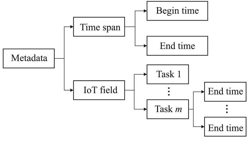
Fig.3 Reconstructing metadata.
4 Experiment and Evaluation
4.1 Data Description
Here, we utilized authentic datasets of the marine observation domain to demonstrate the effectiveness of the proposed AMR. The basic format of these datasets is presented in Table 2.

Table 2 Format of IoT sensor data
The datasets used in this study came from the marine observation system. These datasets were collected in ocean energy-generating test sites in August 2015, represented by a sequence of sensor data containing the sensor information of many ocean observing devices (tasks), such as CTD, wave rider, and so on. The total size of these datasets is around 208 GB.
4.2 Feature Tensor Extraction
-order. For choosing the appropriate Markov Chain order for data preprocessing, we performed several experiments in each potential scenario (Fig.4), in which the greater the degree that the conditional entropy level is, the weaker the representation of preprocessed data. As shown in Fig.4, The third-order Markov algorithm outperforms the lower-order Markov algorithm and only has a slight little difference from the 4-order Markov. Furthermore, as the valueincreases, the hierarchy of the conditional entropy increases accordingly at varying Markov orders. In summary, AMR uses higher-order Markov to obtain higher qualified preprocessed data. Nevertheless, this is consider- ed infeasible due to the additional temporal and quantitative complexity of AMR. Based on Fig.4, we choose=3 to continue our experiment.
Threshold. To choose a properfor AMR, we utilize 20% of marine observation datasets as testing data to calculate both time consumption and success ratio. The correlation between the value ofand time consumption. is shown in Fig.5. As can be seen, AMR’s time consumption becomes higher with the increasing value of; and it is also evident that the time consumption (=10) is much larger than the one when=2. Meanwhile, the success ratios under differentvalues are calculated, and the results are shown in Fig.6. Better performance can be obtained if a higheris chosen until=8. By comparing the average success ratio of=8 and=10, We find that the success ratio decreases whenfrom 8 to 10 upon comparing the average success ratio of=8 and=10. Therefore, we take both time consumption and success ratio into account and choose=8 as the proper parameter to continue our experiment.
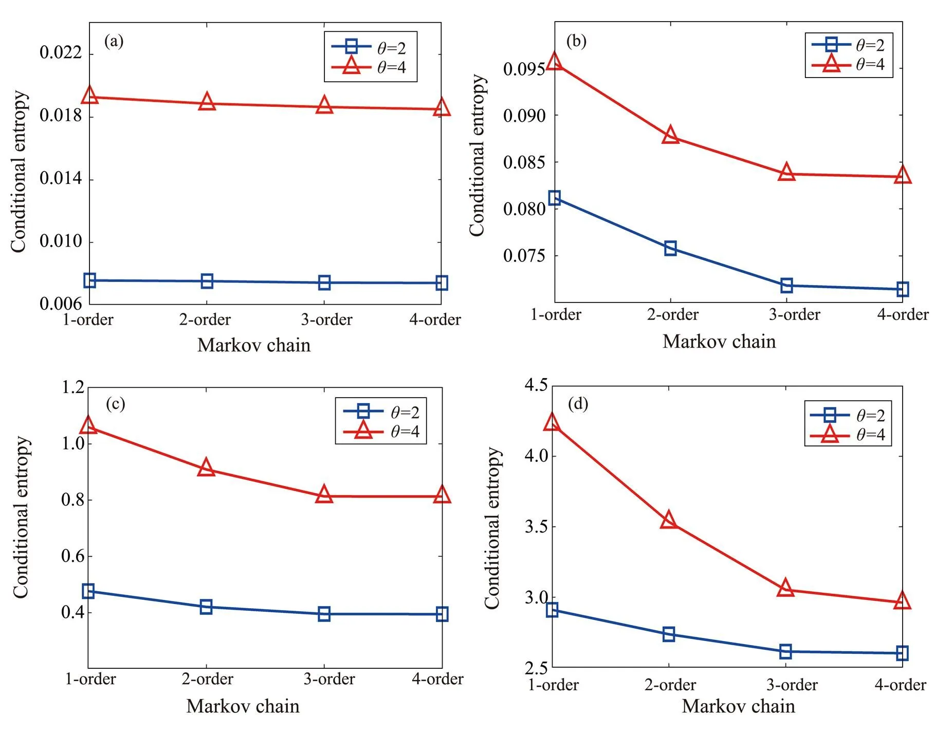
Fig.4 Conditional entropy under k-order Markov.(a), wave buoy; (b), wave rider;(c), CTD;(d), vessel.
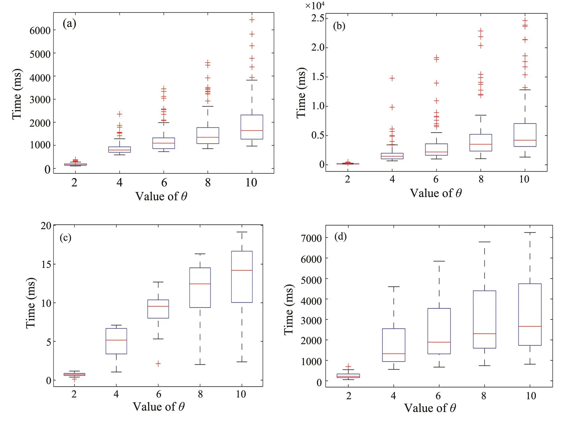
Fig.5 Time consumption at different θvalues with the 3-order Markov function.(a), wave buoy; (b), wave rider;(c), CTD;(d), vessel.
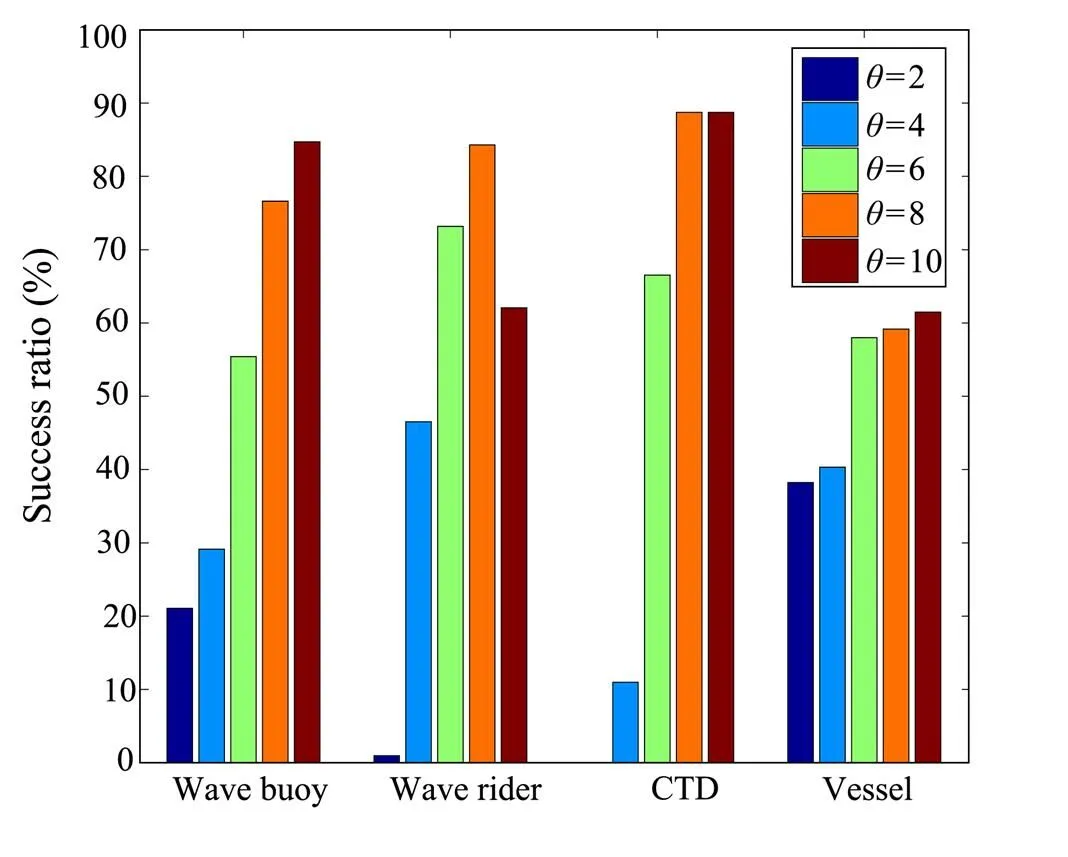
Fig.6 Success ratio at different θwith 3-order Markov function.
Correlation pair ratio. To demonstrate the validity and rationality of the AMR horizontal correlation extraction approach, we conduct trials using real datasets of marine observations. Table 3 presents the extraction results from Algorithm 6. Regarding the numerical distribution, it is evident that the IoT devices CTD and Vessel are analogous.Furthermore, there are relatively large similarities between Wave Buoy and Wave Rider, thereby demonstrating the feasibility of the proposed AMR feature extraction method.
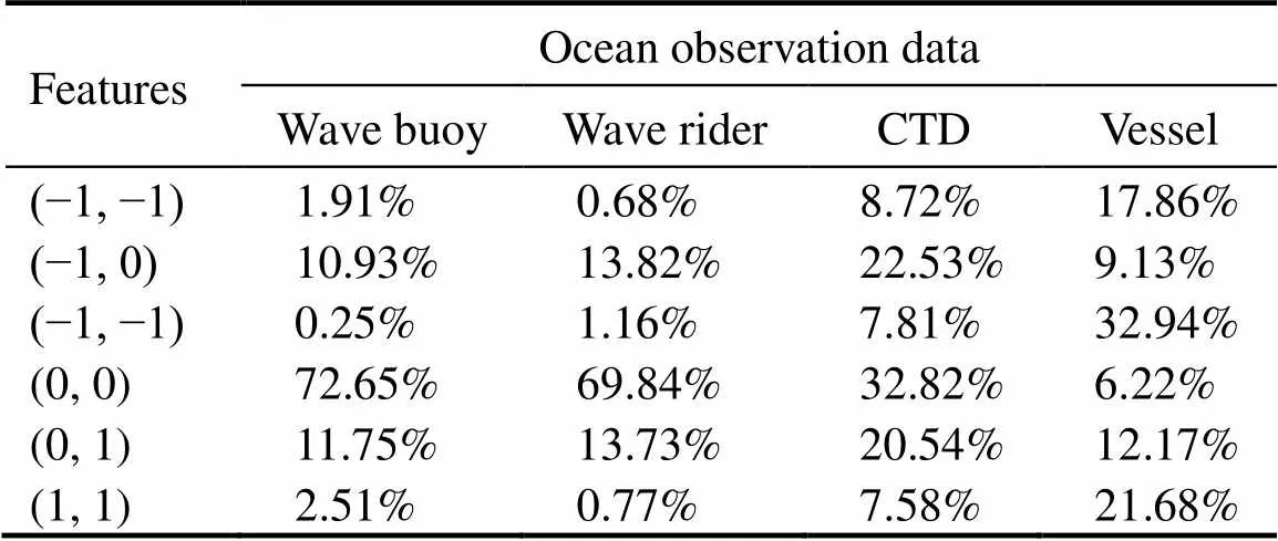
Table 3 Characteristics of household appliances testing data
Algorithm 6: Statistical distribution extraction
Output: Feature tensor

2 Define a correlation pair list;
3 for=0 to+row.count−1 do
5 Count the number of each combination;
6 for=0 to+column.count−1 do
7 for=+1 to+column.count−1do
11 else
14 end
15 end
16 end
17 end
19 Generate feature tensor→=(1,2, ···,v);
20 Return feature tensor
4.3 Recognition Performance
In Section 3, we use the FSFDP algorithm to cluster the feature tensors. In our experiment, two more clustering algorithms are utilized, as shown in Figs.7 and 8. K-means is a standard vector quantization approach to cluster profiling in data mining and (self-organizing) maps (SOM) (Hartigan and Wong, 1979; Mangiameli., 1996). It functions as an artificial neural network employing no-supervised learning to produce a low-dimensional representation of the input space of the training samples, which is also ideal for clustering.
Marine observation task recognition. As shown in Fig.9, we obtain the success ratio using a different method. The results indicate that the success ratio becomes higher and eventually becomes a stable value with the increasing num- ber of testing datasets. In addition, the method of using a 3-order Markov transition probability matrix with FSFDP performs better than any other method.
IoT sensor identification. In this test, we use 30% out of the total datasets as testing material and 70% as training material. Thus, we are able to fulfill the field-aware IoT sensor recognition requirement by leveraging BP neural network as a classification method. Then, we utilize the two metrics below for the evaluation of the perfor- mance of the AMR identification algorithm, thus allowing us to compare the recognition performance with those pre- sented in other related research (SMDD and SPAM):

whereis the right recognition result,is the recognition result from AMR algorithm,is the manual recognition result, andis the wrong recognition result.
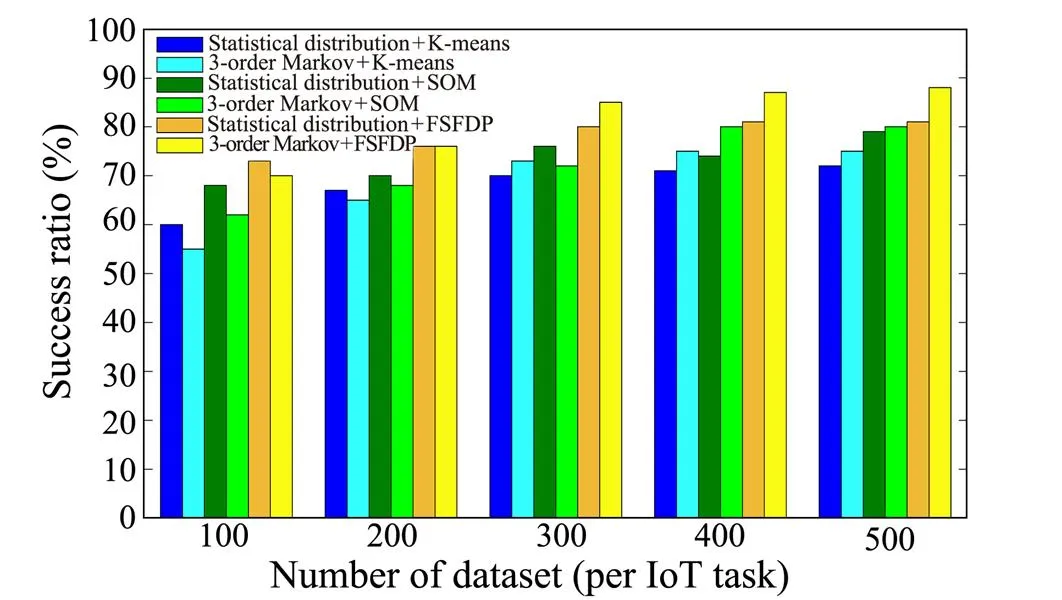
Fig.8 IoT task recognition performance comparison among different methods.
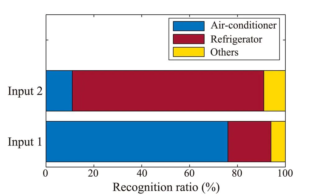
Fig.9 IoT field recognition performance.
5 Related Works
A data lake fulfills the requirement for fast data integration and skips the process of data extraction, conversion, and cleansing, thus satisfying the lasted demand of marineobservation and ample data storage. However, we can only use several research findings for reference. Current data lakes are built is almost exclusively by large commercial enterprises such as Google and Amazon, and this task in- volves advanced infrastructure requirements for tremendous marine data. In addition, only highly qualified data scientists can operate the data lakes instead of data consumers, which slows down the development of data lake technology. Halevy(2016) solved problems from the scale and heterogeneity of Google’s data lake, whereas Terrizzano(2015) from IBM proposed the importance of having a curated data lake. The data should go through a curation process to enhance its availability. Finally, Alrehamy. built a data lake for personal information storage and management, generating data from the Internet.
Although data lakes have their advantages in storing marine observation big data, they may turn into data swamps due to because of invalid metadata management. Resear- chers are devoted to protecting data lakes from transforming into data swamps. In this study, we propose a novel technique based on anchor modeling, which efficiently re- inforces metadata management. Naumann (2014) revealed new research directions and challenges of data profiling for IoT heterogeneous metadata (Ma and Chen, 2016). In particular, data wranglers aim to preprocess the raw marine observation data before loading them into a data lake. This highlights the importance of constructing qualified metadata. However, researchers have seldom contributed to restoring data swamps to data lakes by reconstructing metadata. Thus, in this paper, we use time series analysis techniques to extract meaningful characteristics of raw ma-rine data, which can be utilized to reconstruct metadata for data lakes. Jason et al. achieved automatic sensor recognition through their analysis of the characteristics of data value allocation using the BP neural network. However, this only pertains to one-on-one sensor recognition rather than marine observation tasks. Thus, it is unable to represent the characteristics of big data in data swamps because those data are usually generated by different tasks stored as structured datasets. Time series are utilized to dis-cover temporal patterns for event recognition. Those events are explicitly structured and do not cater to metadata construction.
6 Conclusions and Future Work
This paper proposes an AI-based algorithm called AMR to reconstruct metadata for marine observation data in data swamps. First, we introduce the concept of a data lake, revealing its advantages and disadvantages for raw marine data storage compared with the data warehouse. Then, we present the data swamp problems, such as invalid metadata management. The emergence of such problems has attracted more attention as researchers look for ways tohandle them. Second, we design a data preprocessor for dealing with data in data swamps. We extract the characteristics of marine observation data, treat them as input ten- sors of neural networks, and implement clustering based onthe technology of data mining and machine learning. Through the analysis of preprocessed data, we find the dependence between various sensors within a single observation task and transform it into a geometric model. Third, in terms of clustering outputs, we evaluate the comparability among input IoT sensor data with training clustering outputs. Fina- lly, we use the recognition result to reconstruct metadata, which consist of marine observation field information and task information. Other clustering algorithms will be considered in our future work, and more metadata details will be reconstructed instead of the marine observation field only. Furthermore, we intend tostudy data lakes and data swamps, as well as propose an efficient architecture for marine observation big data storage.
Acknowledgement
The study is supported by the Shandong Province Natural Science Foundation (No. ZR2020QF028).
Alex, R., and Alessandro, L., 2014. Clustering by fast search and find of density peaks., 344 (6191): 1492-1496, DOI: 10.1126/science.1242072.
Alrehamy, H., and Walker, C., 2015. Personal data lake with datagravity pull.Dalian, 160-167.
Atzori, L., Iera, A., and Morabito, G., 2010. The Internet of Things: A survey., 54 (15): 2787-2805, https://doi.org/10.1016/j.comnet.2010.05.010.
Bandyopadhyay, D., and Sen, J., 2011. Internet of Things: Applications and challenges in technology and standardization.,58: 49-69, https://doi.org/10.1007/s11277-011-0288-5.
Bettini, C., Wang, X. S., Jajodia, S., and Lin, J. L., 1998. Discovering frequent event patterns with multiple granularities in time sequences., 10 (2): 222-237, DOI: 10.1109/69.683754.
Datta, S. K., and Bonnet, C., 2015. Internet of Things and M2M communication as enablers of smart city initiatives.. Cambridge, 393-398.
Evans, D., 2011. The Internet of Things: How the next evolution of the internet is changing everything., 1: 1-11.
Golov, N., and Ronnback, L., 2015. Big data normalization for massively parallel processing database.Stockholm, Swe-den,154-163.
Gubbi, J., Buyya, R., Marusic, S., and Palaniswami, M., 2013. Internet of Things (IoT): A vision, architectural elements, and future directions., 29 (7): 1645-1660, https://doi.org/10.1016/j.future.2013.01.010.
Hai, R., Geisler, S., and Quix, C., 2016. Constance: An intelligent data lake system.. San Francisco, 2097-2100.
Halevy, A. Y., Korn, F., Noy, N. F., Olston, C., Polyzotis, N., Roy, S.,, 2016. Managing Google’s data lake: An overview of the Goods system., 39 (3): 5-14.
Hartigan, J. A., and Wong, M. A., 1979. Algorithm AS 136: A K-means clustering algorithm., 28 (1): 100-108, https://doi.org/10.2307/2346830.
Hu, C. Q., Pu, Y., Yang, F., Zhao, R., Alrawais, A., and Xiang, T., 2020. Secure and efficient data collection and storage of IoT in smart ocean., 7 (10): 9980-9994, DOI: 10.1109/JIOT.2020.2988733.
Jackson, K. R., Ramakrishnan, L., Muriki, K., Canon, S., Cholia,S., Shalf, J.,, 2010. Performance analysis of high performance computing applications on the Amazon Web Services Cloud.. Indianapolis, IN, 159-168.
Jiang, F., Ma, J., Wang, B., Shen, F., and Yuan, L., 2021. Ocean observation data prediction for Argo data quality control using deep bidirectional LSTM network., 2021: 1-11, https://doi.org/10.1155/2021/5665386.
Ma, H., and Chen, B., 2016. An authentication protocol based on quantum key distribution using decoy-state method for he- terogeneous IoT.,91: 1335-1344, https://doi.org/10.1007/s11277-016-3531-2.
Mangiameli, P., Chen, S. K., and West, D., 1996. A comparison of SOM neural network and hierarchical clustering methods., 93 (2): 402-417, https://doi.org/10.1016/0377-2217(96)00038-0.
McCrory, D., 2010. Data gravity in the clouds. https://datagravitas. com/2010/12/07/data-gravity-in-the-clouds/.
Miorandi, D., Sicari, S., Pellegrini, F. D., and Chlamtac, I., 2012. Internet of Things: Vision, applications and research challenges., 10 (7): 1497-1516, https://doi.org/10.1016/j.adhoc.2012.02.016.
Naumann, F., 2014. Data profiling revisited., 42 (4): 40-49, DOI:10.1145/2590989.2590995.
O’Leary, D. E., 2014. Embedding AI and crowdsourcing in the big data lake., 29 (5): 70-73, DOI:10.1109/MIS.2014.82.
Qiu, Z., Hu, N., Guo, Z., Qiu, L., Shuai, G., and Xi, W., 2016. IoT sensing parameters adaptive matching algorithm.. Shenyang, 198-211.
Satija, D., Bagchi, M., and Martínez-Ávila, D., 2020. Metadata management and application., 58 (4): 84-107, DOI:10.5958/0976-2469.2020.00030.2.
Sawadogo, P. N., and Darmont, J., 2020. On data lake architectures and metadata management., 56 (1): 97-120, DOI:10.1007/s10844-020-00608-7.
Terrizzano, I. G., Schwarz, P. M., and Colino, J. E., 2015. Data wrangling: The challenging Yourney from the wild to the lake.Asilomar, California.
Vassiliadis, P., Simitsis, A., and Skiadopoulos, S., 2002. Conceptual modeling for ETL processes.. McLean Virginia, USA, 14-21.
Wu, Y., Zhu, Y., and Li, B., 2014. Trajectory improves data delivery in urban vehicular networks., 25 (4): 1089-1100, DOI:10.1109/TPDS.2013.118.
Xu, G., Shi, Y., Sun, X., and Shen, W., 2019. Internet of Things in marine environment monitoring: A review., 19 (7): 1717, DOI:10.3390/s19071711.
Xu, H., 2020. Classification and storage method of marine multi-source transmission data under cloud computing., 115: 84-86, DOI:10.2112/JCR-SI115-025.1.
You, L. I., and Liu, D. B., 2005. A method for automatic schema matching using characteristic of data distribution., 32 (11): 85-86.
(May 20, 2022;
October 9, 2022;
February 27, 2023)
© Ocean University of China, Science Press and Springer-Verlag GmbH Germany 2023
. E-mail: guoshuai@qut.edu.cn
(Edited by Chen Wenwen)
 Journal of Ocean University of China2023年6期
- Journal of Ocean University of China的其它文章
- Effects of 5-Azacytidine (AZA) on the Growth, Antioxidant Activities and Germination of Pellicle Cystsof Scrippsiella acuminata (Diophyceae)
- Improving Yolo5 for Real-Time Detection of Small Targets in Side Scan Sonar Images
- Wave Radiation by a Floating Body in Water of Finite Depth Using an Exact DtN Boundary Condition
- Underwater Acoustic Signal Noise Reduction Based on a Fully Convolutional Encoder-Decoder Neural Network
- Revisiting the Seasonal Evolution of the Indian Ocean Dipole from the Perspective of Process-Based Decomposition
- Assessment of Storm Surge and Flood Inundation in Chittagong City of Bangladesh Based on ADCIRC and GIS
