Deep learning framework for time series classification based on multiple imaging and hybrid quantum neural networks

Jianshe Xie(谢建设) and Yumin Dong(董玉民)

College of Computer and Information Science,Chongqing Normal University,Chongqing 401331,China

Keywords: quantum neural networks,time series classification,time-series images,feature fusion

1.Introduction

A time series is a series of data points (measurements)with a natural time order.Many important real-world pattern recognition tasks involve time series analysis.Time series are prevalent in various fields, such as biology, astronomy, meteorology,finance,medicine,engineering,and others.[1]People use techniques such as classification, segmentation, and prediction of time series to exploit their potential value as much as possible.TSC, as a branch of time series analysis, has attracted a lot of attention in the field of data mining.

Time series data are highly volatile and uncertain, and traditional methods such as expert empirical consultation and multiple models perform poorly in classification.In recent years, a large number of algorithms have been developed for TSC,which can be specifically summarized as distance-based time series classification algorithms and feature-based classification algorithms.The most popular distance-based algorithms are the nearest neighbor (NN) classifier and distance function,[2]thek-nearest neighbor (k-NN)[3]and dynamic time warping(DTW).[4]In the feature-based algorithm,Nanopoulos uses mean,standard deviation,skewness,and kurtosis to represent and classify time series,[5]and Morchenet al.used features derived from wavelet and Fourier transforms of a series of time series datasets to classify time series.[6]Subsequently,Linet al.[7]proposed the bag-of-words(BOW)method,which quantifies the extracted feature BOW and feeds it into the classifier as a feature attribute.

Recently, DL models have achieved high recognition rates in computer vision recognition.DL is practical and effective in generating features of raw data,which provides clues to improve the accuracy of TSC methods.The idea of converting time series to images and using them as input for deep learning has received a lot of attention.Convolutional neural networks(CNN),one of the most successful DL models,have been applied to solve complex problems in many fields.A CNN unifies the feature learning and classification parts in one model and learns them jointly.As a result,CNN has achieved remarkable success in image and video recognition tasks.

Quantum machine learning(QML)[8]combines classical machine learning techniques with quantum computing and is emerging as a powerful approach that allows quantum acceleration and improvement of classical machine learning algorithms.QML mainly uses parametric quantum circuits(PQC)for prediction and classification.Quantum circuits for machine learning problems are similar to classical neural networks (NN), so they are sometimes called QNN.The input layer of a QNN is called the embedded circuit and the hidden layer is called the variable quantum circuit layer, which together form the PQC.So far,several QML algorithms have been proposed and demonstrated, including quantum support vector machines,[9,10]quantum deep learning,[11-17]quantum Boltzmann machines (QBM),[18,19]and quantum generative adversarial learning.[20-22]Exploration of quantum computing has shown that quantum effects,such as superposition and entanglement,can improve the efficiency of training when solving certain problems.

Inspired by recent achievements in computer vision techniques and quantum machine learning, we propose a framework for learning based on multiple imaging and hybrid quantum neural networks.Specifically,the time series datasets are first divided into two categories,one with a sufficient number of training samples and the other with an insufficient number of samples.For the former, we use recurrence plots (RP)[36]to convert the raw temporal data into 2D images.For the latter,we will use four time series imaging methods,RP,Markov transition field (MTF),[38]Gramian angular summation field(GASF),[25]and Gramian angular difference field(GADF),[25]to convert the time series into four 2D images.Then, the four images are fused into one image to strengthen the features and reduce the probability of overfitting in the training process caused by insufficient sample quantity.The resulting images will be trained and classified by combining QNN and classical neural networks.ResNet[24]is used as the feature extractor,and QNN is used as the classifier.In order to evaluate the influence of different quantum variational circuits on classification, we will use four kinds of quantum circuits as classifiers.The results show that compared with the three most recent best classification methods, our approach achieves the best performance on 9 of the 10 standard datasets in the UCR archive.[39]In datasets with a small number of samples,experiments showed that the method using four time series imaged and fused achieved the best performance on four of the standard datasets from the UCR archive compared to the method using a single time series imaged.

The main contributions of this paper are summarized in the following three points.First, for the TSC task, a model combining time-series imaging and hybrid quantum neural networks is proposed.Second, considering the insufficient sample size of the training data, four time-series imaging fusion methods are used to enhance the sample features and reduce the risk of overfitting.Third, to explore the impact of quantum circuits,four quantum circuits were designed and investigated for the TSC task.

The rest of this paper is organized as follows.In Section 2, we discuss the background and related work.We present our framework in Section 3,and give the experimental results of the proposed method on a standard dataset in Section 4.Finally,Section 5 presents the conclusion and perspectives.

2.Related work

In recent years, DL has made impressive progress in many areas, including speech recognition, image recognition, and natural language processing, which has motivated researchers to study DL in the TSC domain.It is only recently that deep learning methods such as multi-scale convolutional neural networks (MCNN),[23]fully convolutional networks (FCN),[24]and ResNet[24]have started to appear in TSC.Wang[25]proposed converting time series into images using GAF and MTF and applying CNN models for time series classification(GAF-MTF)in 2015.Subsequently,Hatami[26]et al.proposed the use of RP to convert time series into 2D texture images and then perform recognition operations using a deep CNN classifier(RPCNN).Chen[27]et al.investigated a relative position matrix to convert time series data into 2D images and construct an improved CNN architecture to classify the data (RPMCNN).Karim,[28]on the other hand, proposed solving the TSC problem with long short-term memory fully convolutional networks (LSTM-FCN).These approaches can be broadly classified into two categories: one relies on modified traditional CNN architectures and uses 1D time series signals as input, such as LSTM-FCN, while the other first converts the original time series into 2D images and then applies them to deep learning models, such as GAF-MTF, RPCNN,and RPMCNN.

Quantum computing (QC) on the other hand, as a new computing paradigm, is expected to be applied in several fields, including machine learning.The field of QC has demonstrated its important role in problems that are difficult to solve by their classical counterparts through quantum superiority.[29,30]The quantum algorithm for deep convolutional neural networks proposed by Kerenidis[31]implements a new frontier in image recognition and numerical simulations of MNIST dataset classification,demonstrating the efficiency of quantum computing.In Ref.[32],a hybrid quantum convolution neural network model is introduced to predict COVID-19 images.It fully exploits the advantages of quantum convolutional layers and CNN and demonstrates the possibility of hybrid quantum models for new crown image classification.Mari[33]proposed a migration learning model in hybrid classical-quantum neural networks to demonstrate the possibility of quantum migration learning.Mari used the ResNet deep learning model to process the samples classically and then used a variational quantum circuit to process the features.There are several classical feature extraction models to choose from, such as AlexNet,[34]ResNet,[24]DENSENET,[35]and VGGNet.[36]The feature extraction in our proposed model is also based on the ResNet model to solve the TSC task.

However,there are few studies based on using time-series imaging and hybrid quantum neural networks to solve TSC tasks.Most of the existing hybrid quantum neural network models have mostly focused on solving predictive classification tasks where the original data are images and have not explored the possibilities of hybrid quantum models for processing secondary images.Our proposed model proves its possibility and,in experiments on the UCR archive,it is found that the hybrid model can achieve an accuracy equal to or even better than the classical model for the classification of time-series imaging data compared to several best models.

3.Methodology

3.1.MIHQNN framework

The overall architecture of the MIHQNN is shown in Fig.1, which consists of three sequential phases: the imaging phase,feature extraction phase,and classification phase.

1.In the imaging stage, we classify the dataset into two types, one with sufficient sample data and the other with insufficient sample data.The former applies the RP time series imaging method alone to transform a one-dimensional time series into a 2D image, and the latter uses four time series imaging methods and fuses them into a single image.

2.In the feature extraction phase,we will use a modified ResNet model.This includes several residual blocks and fully connected layers to output the extracted features.

3.In the classification phase,we designed four classifiers based on quantum circuits for each dataset, and trained and tested them for 50 iterations.

See Subsections 3.2-3.4 for more details.the feature fusion method, the four sets of feature vectors are combined into a joint vector, thus extending the feature vector space of the original image,which is beneficial to the deep learning framework for its classification and thus improves the classification rate.Multiple imaging and fusion, specifically four imaging methods,RP,MTF,GASF,and GADF,are used to convert each time series into four images.And an image is formed by RP,MTF,GASF,and GADF in a counterclockwise direction, which can be seen in Fig.2.The principles of the four time series imaging are described in detail below.

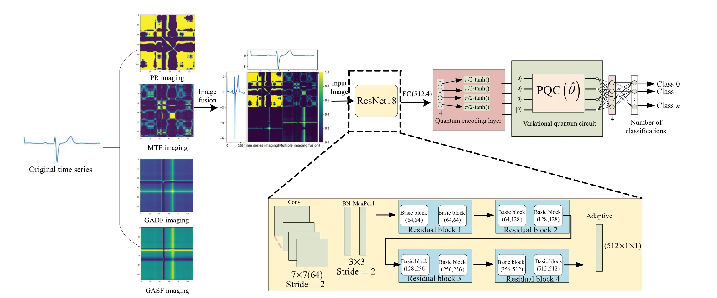
Fig.2.MIHQNN model based on multiple time series imaging fusion.

3.2.Imaging stage

For datasets with a sufficient number of samples,we use a single RP imaging,because with a sufficient number of samples,the MIHQNN model rarely over-fits during training.The use of multiple imaging fusions may add additional consumption, including time and memory consumption.However, for datasets with insufficient sample size, the need to use multiple imaging becomes apparent.The edges and diagonals of time series images contain richer classification features.Using

3.2.1.RP imaging

RP is an important method for analyzing the periodicity,chaos,and non-stationarity of time series.It can be used to reveal the internal structure of time series,giving a priori knowledge about similarity,informativeness,and predictability.RP is particularly suitable for short time series data, and can test the smoothness and intrinsic similarity of time series.RP is an image that represents the distance between trajectories extracted from the original time series,as follows.

Given the time series (x1,...,xn), the result of reconstructing the time series is

wheremdenotes the embedding dimension andτdenotes the delay time.

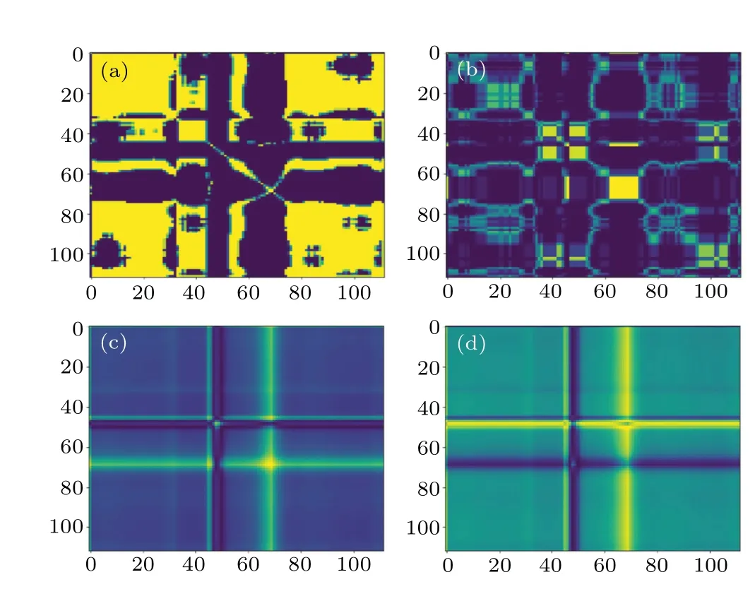
Fig.3.Applying RP,MTF,GASF,and GADF to convert time series to images.

The distance between pointi,xi, and pointj,xj, in the reconstructed phase space is

The recursive value can then be expressed as

whereθrepresents the Heaviside function, a segmentation function that is commonly used in recursive graphs to represent the stopping conditions of recursion.εis a threshold; if“none”,the graph is repeated without binarization.If“point”,the threshold is calculated,e.g.,the percentage of points is less than the threshold.If “distance”, then the threshold is calculated as the maximum distance.This is set to “none” when plotting RP in this article.

Figure 3(a)shows the image after applying RP to a time series transformation,whereτ=0.1 andm=1.

3.2.2.MTF imaging

MTF is proposed based on the first-order Markov chain transformation because Markov transfer fields are insensitive to the time dependence of the sequences,so MTF is based on the relationship of time positions.

The process of constructing the MTF is as follows.

Step 1: First divide the time series data intoQbins.Each data pointicorresponds to a unique bin, i.e., each data point has only one identifierqi,i ∈{1,2,...,Q}.

Step 2: Construct a Markov state transfer matrix

whereAijrepresents the transfer probability of stateitransforming to statej.The transfer probability is generally estimated using the maximum likelihood method, where the matrix size is[Q,Q].

Step 3:Construct the Markov variation fieldM.Mis anN×Nmatrix andNis the length of the time series,

whereqkis the bin ofxk,qlis the bin ofxl, andxis the time series data.

The shape of the MTF is as follows:

Figure 3(b)shows the image after applying MTF to a time series transformation,where bins=5.

3.2.3.GAF imaging

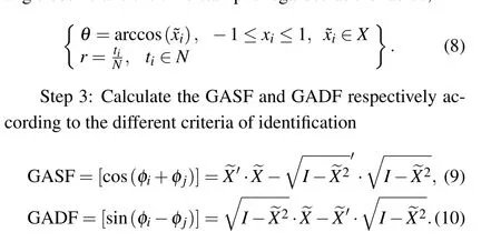
A GAF image is an image obtained from a time series,mainly based on some temporal correlation between each pair of values starting at a given time.There are two methods:GASF and GADF.The difference between these two methods is that, when the scaled time series data are converted from a right angle coordinate system to a polar coordinate system,GASF considers the sum of the angles between different points as a criterion for identifying different points in time and GADF considers the difference in angle between different points as a criterion for identifying different time points.The steps of the GAF implementation are as follows.

Step 1: Scale the data to [-1,1] (in this paper we scale the data to [-1,1]; we can also scale the data to [0,1]).The formula for scaling is

whereXrepresents a time series data.

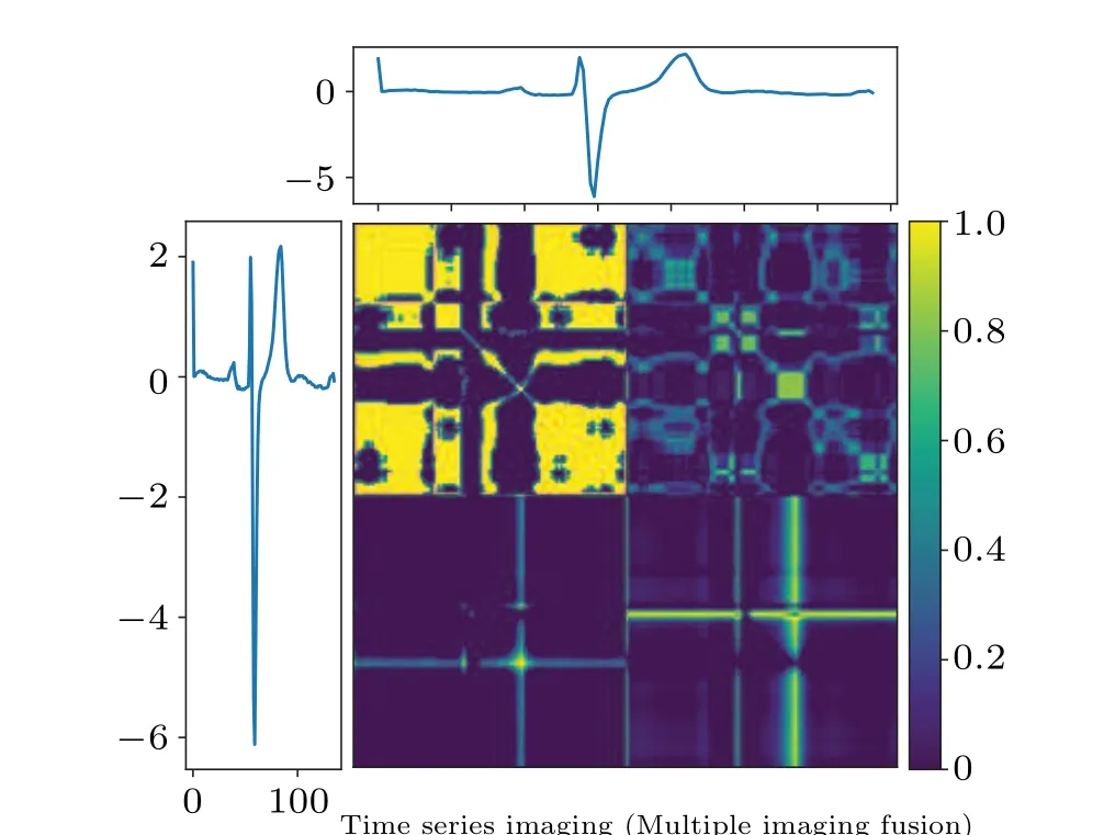
Fig.4.Feature fusion of combined images.In order to solve the problem of single image feature loss during MIHQNN training and classification,the combined image algorithm converts the time series into four images and combines them into a square image for feature-level fusion.The combined images are RP,MTF,GASF,and GADF from top left to bottom right.

Step 2: Convert the scaled sequence data to polar coordinates, i.e., the value ～Xof the time series is regarded as the angle cosine and the time stamp is regarded as the radius,

Figures 3(c)and 3(d)show the images after applying the GASF and GADF to transform the time series.Figure 4 shows the shape after fusing the four images.

3.3.Feature extraction stage

After the raw time series data have been converted into images,CNN models can be trained to perform feature extraction on these images,and the feature extraction model in this paper is based on ResNet for improvement.The main purposes of the modification are:1)Some mature deep learning models,such as ResNet,are commonly used for RGB(three-channel)color image classification tasks.However,after the processing in Subsection 3.2, the obtained image type is single channel,and the input channel of the first convolution layer needs to be modified to single channel.2)The output of the feature extraction model must be consistent with the input requirements of the later classification stage.In this paper,the trainable parametric variational quantum circuit used as the classification stage is 4 qubits in number,so it is necessary to set the number of features of the output of the feature extraction model to 4.

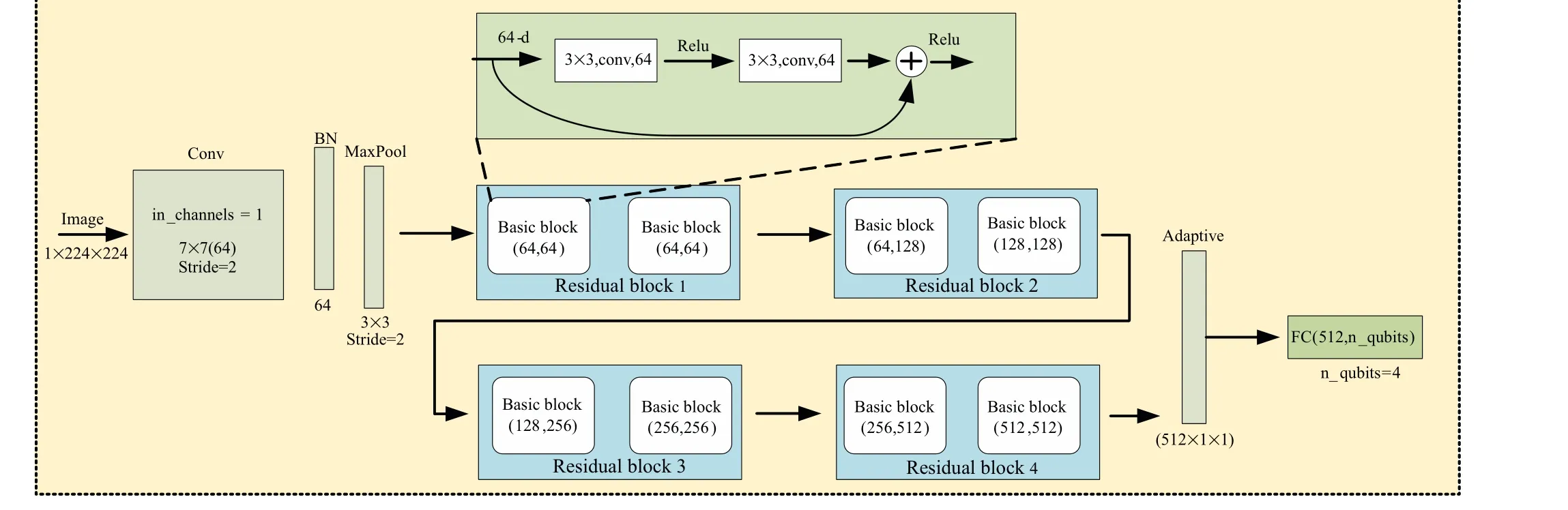
Fig.5.Time series data feature extraction model.

As shown in Fig.5,the feature extraction model contains three main components.The composition of the first part: a 1-channel input of size 224×224 with 64 output channels, a 7×7 convolutional layer (conv) of step size 2 followed by a batch normalization layer(BN),followed by a 3×3 maximum pooling layer(MaxPool)of step size 2.BN is mainly used to solve the gradient disappearance and gradient explosion problems.The composition of the second part: it mainly contains four residual blocks,each with two 3×3 convolutional layers with the same number of output channels inside.Each convolutional layer is followed by a batch planning layer and a ReLU activation function.The input also needs to be added directly before the final ReLU activation function in each residual block.Such a design can satisfy the requirement that the outputs of the 2 convolutional layers have the same shape as the inputs, so that they can be added together.The composition of the third part: finally, the features extracted from the residual layer are followed by a global average pooling, and the global average pooling is added to suppress the overfitting phenomenon.Then a fully connected layer is added to match the input dimension of the subsequent quantum neural network classifier.

3.4.Classification stage

In the classification phase,we focus on exploring the correlation between the possibility of using quantum classifiers instead of classical classifiers and the classification accuracy of different quantum circuits.The classification phase has two main components: 1) The features obtained after the feature extraction stage are classical states, which cannot be directly embedded in the quantum circuit at this point, and must go through an encoding section where the extracted features are fed into the quantum variational circuit.2) Quantum circuits are the basis of quantum neural networks.In quantum neural networks,quantum circuits are used to build neurons and layers,while the training and optimization of neural networks are achieved by adjusting the parameters of quantum gates.Both the design and optimization of quantum circuits affect the efficiency and performance of quantum neural networks.Once the features were input,we used four quantum circuits as four classifiers each to explore the effect of different quantum circuits on the classification performance.

3.4.1.Encoding stage

In order to construct hybrid quantum models, it is crucial to convert classical data to a high-dimensional quantum representation.Ground state coding,[43]amplitude coding,[43]angle coding,[43]IQP coding,[44]and Hamiltonian evolution coding[45]have been proposed.The encoding approach we take is to convert the previously obtained eigenvalues into angles,as in Fig.1,by multiplying each of the four eigenvalues by(π/2), and then applying them to the quantum circuit.As in Fig.6(a),the Hadamard gate(H)can be applied first to act on the initial quantum state, placing the initial quantum state in the superposition state.The RY gate is then applied to the qubit,and the control angle of the RY gate is the angle previously converted by the eigenvalue,which enables the transfer of the obtained classical information to the subsequent quantum circuit.

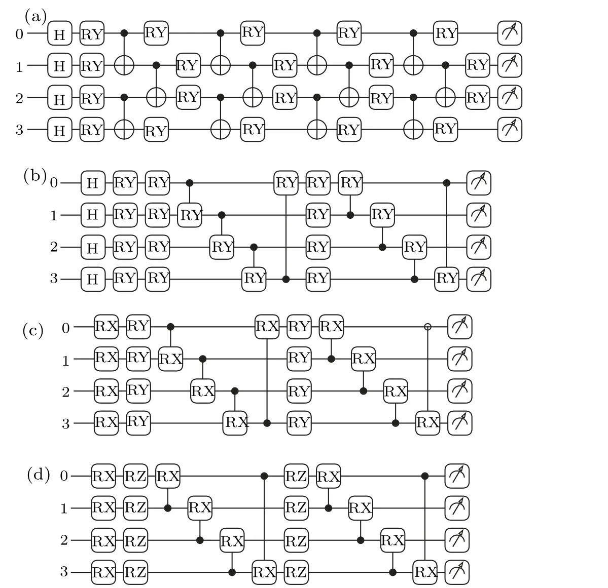
Fig.6.Parametric quantum circuits.(a)Circuit 1,four qubits and four layer confgiuration.(b)Circuit 2,four qubits and single layer confgiuration.Mainly composed of the RY gate.(c)Circuit 3,four qubits and single layer confgiuration.Mainly composed of the RX gate.(d) Circuit 4,four qubits and two layer confgiuration.

3.4.2.Quantum circuit classification stage

To create MIHQNN,parametric quantum circuits need to be used as the hidden layer of the neural network, and four types of circuits are selected and designed in this paper.A description of the circuit employed will help provide insight into how the quantum gate affects the final result.Figure 6(a)related configurations are described here and presents more information about the quantum circuit.[40]

In Fig.6(a), each qubit first gets a superposition state through the H gate and then through the RY gate, the parameters of which are the outputs of the classical network.Then CNOT gates are used to entangle with each other,where the RY gates that pass through are constant rotation, i.e.,Ry(θi)=I,i=0, 1, 2, 3.Then the state before the CNOT gate is

Because the RY gate is assumed to be a constant rotation here, the state|ψ1〉 remains unchanged after passing through the CNOT gate, i.e.,|ψ2〉=|ψ1〉.The effect of RY gates in the real situation is not constant rotation, which reflects the importance of encoding classical information into quantum information and feeding it into the quantum circuit.Then the state after passing through the revolving door four times is

The depth of circuit 1 is 4.The combination of the CNOT gate and the RY gate is repeated a total of four times.During training the parameterθjis also called quantum weight,similar to the weights in neural networks,andθjis trainable.The principles of circuit 2, circuit 3, and circuit 4 are the same as those of circuit 1,except that the combination and depth of the quantum gates are different, in analogy to the different network structures in neural networks.After the superposition and entanglement of the quantum circuit, etc., the final measurement needs to be obtained, and we use the PauliZ-gate at four qubits.The circuit needs to repeat the measurement,and the number of repetitions set in this paper is 1000.The number of measurements obtained is 4.It is also necessary to link a fully connected layer after the quantum circuit;the input of the fully connected layer is 4 and the output isn, wherendenotes the number of targets for classification.The follow-up experiments focus on testing datasets with a target number of 2 or 3 in the UCR archive.

With the whole MIHQNN framework established, we conducted comprehensive experiments, and the results are shown in Section 4.

4.Experiment

4.1.Experimental setup

We evaluated the performance of MIHQNN on a dataset of UCR time series classification archives, of which 14 datasets were selected, with the number of classifications of 2 and 3.

In the subsequent sections, a number of experiments are performed.1) Experiments on four different quantum circuits.2) Experiments on three classical deep learning models(ResNet,DENSENET,VGGNet)for comparison with MIHQNN.3)For MIHQNN,RP time series imaging is compared with multiple time series imaging fusions.

Our proposed MIHQNN is implemented based on Py-Torch and pennylane and runs on an NVIDIA GeForce GTX 1650 graphics card with 896 cores and 4 GB of global memory.The hyperparameters of the model are{batch-size=10,lr=0.0007,step-size=10,gamma=0.1},which denote the batch size,learning rate,learning rate adjustment period, and multiplication factor for updating the learning rate,respectively.The learning rate adjustment period and the learning rate multiplication factor indicate that the learning rate is adjusted to lr×gamma every 10 epochs.For the four MIHQNN classifiers, the Adam optimizer was used to train 50 cycles, regardless of whether the quantum circuits were different, and cross-entropy was chosen as the loss function.The three deep learning models are in the same conditions and environment as MIHQNN.

In this paper,the performance of all TSC methods is evaluated by the classification accuracy,which is defined as

where TP indicates the number of predicted results that agree with the true results,and FN indicates the number of predicted results that do not agree with the true results.

4.2.Comparison with the classical model

To evaluate the performance of MIHQNN,we chose three models that have excelled in processing images and time series in the last five years, ResNet18, DENSENET121, and VGGNet11.They are all three deep learning models based on PyTorch implementation.The number of parameters of the quantum neural network used as the classifier in the MIHQNN model is 2062, while the number of parameters of the classifiers of the three classical models ResNet18,DENSENET121,and VGGNet11 are 513000, 1025000, and 1236428, respectively.In the comparison with the classical model, 10 standard datasets from the UCR archive were selected.The raw time series data are first transformed into 2D images based on RP imaging, and then fed into our model and comparison model for training and testing,respectively.After 50 cycles of training, the best classification accuracy that each model can achieve is collected.

Table 1 shows the accuracy of our proposed method and other TSC methods.It also shows the descriptive information of each dataset{c,Ntr,Nte,L}, which indicate the number of categories,the number of training sets,the number of test sets,and the length of the time series of the dataset, respectively,and where MIHQNN1 represents the MIHQNN model implemented based on circuit 1.

The results in Table 1 show that the MIHQNN model can achieve the same or even better accuracy than the classical model when faced with the TSC task.For example, the MIHQNN model based on quantum circuit 1 achieves the best performance on 3 of the 10 standard datasets archived at UCR.The MIHQNN model based on quantum circuit 2 achieves the best performance on 2 of the 10 standard datasets archived at UCR.In addition, in the experiments on the dataset Small-KitchenAppliances, the accuracy of MIHQNN based on four different quantum circuits is 0.874, 0.832, 0.834, and 0.840,respectively,while the classical models(ResNet,DENSENET,VGGNet) have accuracies of 0.813, 0.792, and 0.781.In the case where the number of trainable parameters of the MIHQNN model is much less than the three classical models mentioned above, the MIHQNN model can achieve the same or even better accuracy than the classical model when faced with the TSC task.This fully demonstrates the feasibility and effectiveness of the hybrid quantum model to deal with time series data, proving its high theoretical and practical value,and it is expected to become one of the tools for time series data analysis in the future.

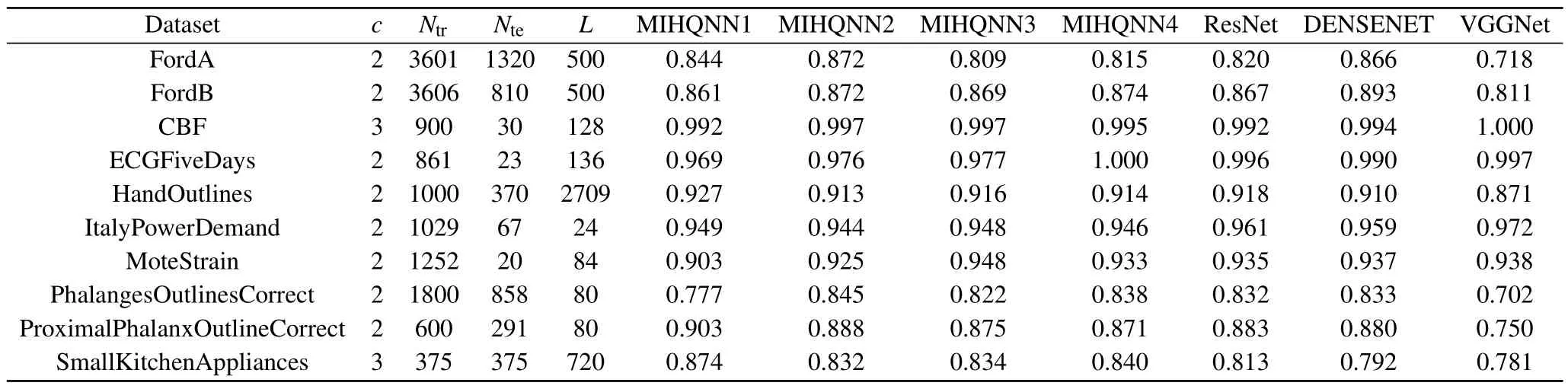
Table 1.Performance(in terms of accuracy)of the proposed method on 10 selected datasets from the UCR archive compared to the prior art TSC algorithm.

4.3.Comparison between four different quantum circuits

For this experiment,we selected four variational quantum circuits as classifiers, each with the same encoding stage and the same initial parameters for each type of revolving gate.As shown in Fig.6,all circuits are one layer,except for circuit 1,which has a four layer structure.circuit 1 and circuit 2 each incorporate four H gates between the initial state and the embedded classical information,while circuit 3 and circuit 4 embed the classical information directly after the initial state.By examining the data in Table 1,it is found that the model based on quantum circuit 1 achieves the best performance on three datasets, HandOutlines, ProximalPhalanxOutlineCorrect and SmallKitchenAppliances.The model based on quantum circuit 2 achieves the best performance on two datasets, FordA and PhalangesOutlinesCorrect.The models based on quantum circuits 3 and 4 both achieve the best performance on only one dataset.This suggests that quantum circuits 1 and 2 may be better suited to handling the TSC task.The reason for this different performance may be that the first two circuits insert a layer of H gates between the classical data embedding layer and the initial state.The H-gate can transform the initial state into a superposition state.A 4 qubit initial state passing through four H-gates will form a system with 42= 16 states existing simultaneously.So the overall effect of the classification is better compared to the quantum circuit without Hgate processing.It also shows that the design and selection of quantum circuits are important when using hybrid quantum neural networks to handle TSC tasks.The layout of qubits in the quantum circuit,the choice of quantum gates,and the optimization will affect the efficiency and performance of the circuit,which has been studied extensively by several researchers in the past.[41,42]

4.4.Comparison between different time series imaging methods

limited by the number of qubits,the number of classifications in the classification datasets targeted in the experiments of this paper is between 1 and 4.Some of the datasets in the UCR archive are too sparse in the number of training samples, causing the selected datasets to be prone to overfitting during the training process.For datasets with sparse data sample sizes, we propose the use of multiple time series imaging fusion methods instead of single RP time series imaging.A time sequence will be converted into a 56×56 2D image by RP, MTF, GASF, and GADF respectively, and then the four images will be fused into a 224×224 image.To validate the possibility of the idea, we selected four datasets in the UCR archive and tested the accuracy of RP-based MIHQNN and MIHQNN based on multiple imaging fusions,as shown in Tables 2 and 3.

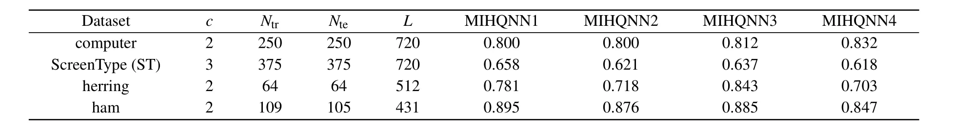
Table 2.Accuracy of RP time-series imaging-based MIHQNN models for datasets with few samples.

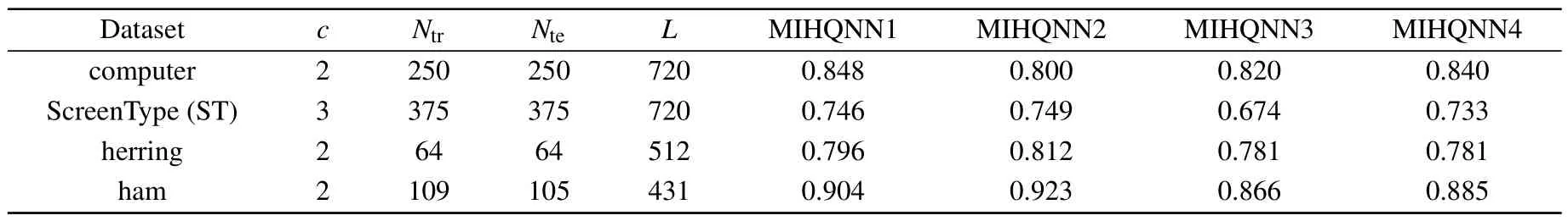
Table 3.Accuracy of MIHQNN models based on multiple time series imaging and fusion for datasets with a small number of samples.

Via observing Figs.7-10, Tables 2 and 3, for the four datasets with sparse sample sizes, the improvement in classification accuracy of MIHQNN based on multiple time series imaging and fusion can be found to be significant compared to MIHQNN based on single RP time series imaging.This is predictable because using multiple imaging and fusion will result in more features, especially at the diagonal bringing together the features of the four images.Multiple imaging and fusion are not necessary, and for sufficiently large sample sizes, using multiple imaging adds additional overhead,such as memory consumption and longer training times.But the idea of multiple imaging and fusion is feasible and valid for particular datasets.And in Figs.7-10, the performance of the multiple imaging fusion-based model is smoother on the test set,which can indicate that the multiple imaging fusion model has better ability to generalize and mitigate the overfitting phenomenon.

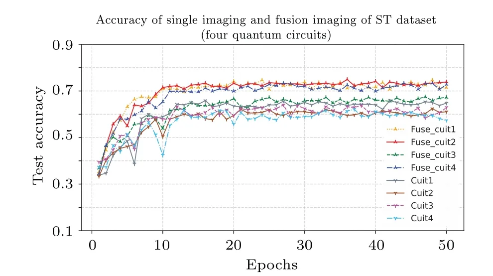
Fig.7.Classification accuracy of four MIHQNN models based on RP and multiple imaging for dataset ST.

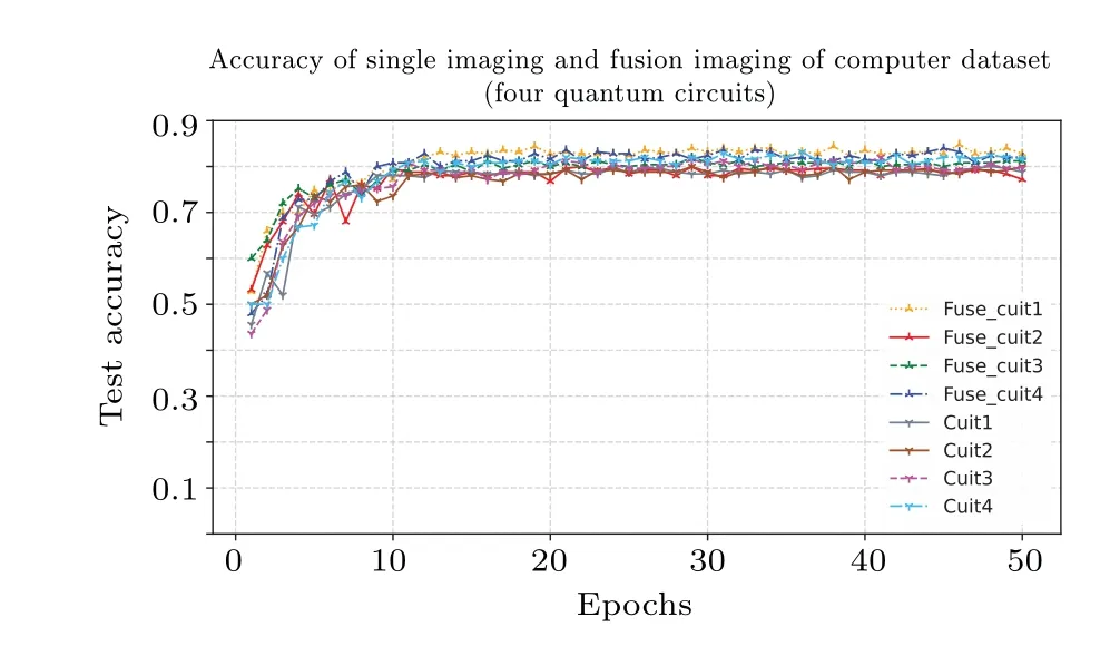
Fig.8.Classification accuracy of four MIHQNN models based on RP and multiple imaging for dataset computer.

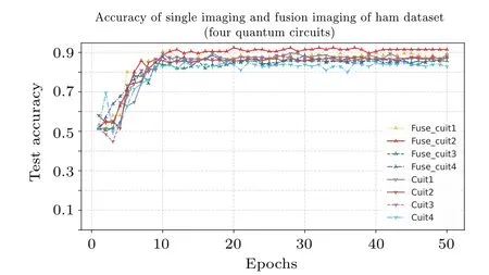
Fig.9.Classification accuracy of four MIHQNN models based on RP and multiple imaging for dataset ham.

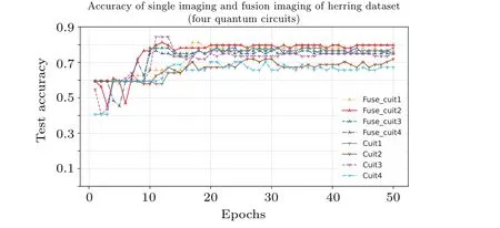
Fig.10.Classification accuracy of four MIHQNN models based on RP and multiple imaging for dataset herring.

Through the above combined comparison,we validate the usability of the approaches based on time series imaging and hybrid quantum neural networks.In particular, the proposed new framework, MIHQNN, was tested in the UCR archive,demonstrating its remarkable performance as well as proving the possibility of the new framework handling TSC problems.

5.Conclusions

We propose a new framework MIHQNN for the TSC task,using a hybrid quantum neural network architecture to recognize 2D images transformed from time series data.Images are converted according to the size of the training samples in the dataset;large samples will be converted by a single RP imaging, and those with small sample sizes will be converted by multiple imaging and fusion.Converting time series to 2D images makes it easier to see similarities in categories from the converted images.In particular, DL has recently been effective in image recognition, and we use a combination of deep learning frameworks and quantum neural networks in order to achieve the best classification results.A number of datasets from the UCR archive were tested and compared with several of the best recent TSC methods.The experimental results prove that MIHQNN performs better overall.

We also separately examined the effect of different quantum circuits on the classification of MIHQNN, as well as the effect of single RP imaging and multiple imaging fusions on the classification of MIHQNN.This research highlights the potential of applying quantum computing to TSC and provides the theoretical and experimental background for future research.

Acknowledgements

Project supported by the National Natural Science Foundation of China (Grant Nos.61772295 and 61572270), the PHD foundation of Chongqing Normal University (Grant No.19XLB003), and Chongqing Technology Foresight and Institutional Innovation Project (Grant No.cstc2021jsyjyzysbAX0011).