ENTIRE SOLUTIONS OF LOTKA-VOLTERRA COMPETITION SYSTEMS WITH NONLOCAL DISPERSAL∗

(郝玉霞) (李万同)

1. School of Mathematics and Statistics, Lanzhou University, Lanzhou 730000, China

2. College of Mathematics and Statistics, Northwest Normal University, Lanzhou 730070, China

E-mail: haoyx15@lzu.edu.cn; wtli@lzu.edu.cn

Jiabing WANG (王佳兵)

School of Mathematics and Physics, Center for Mathematical Sciences, China University of Geosciences, Wuhan 430074, China

E-mail: wangjb@cug.edu.cn

Wenbing XU (许文兵)

School of Mathematical Sciences, Capital Normal University, Beijing 100048, China

E-mail: 6919@cnu.edu.cn

Abstract This paper is mainly concerned with entire solutions of the following two-species Lotka-Volterra competition system with nonlocal (convolution) dispersals:Here a ≠ 1, b ≠ 1, d,and r are positive constants.By studying the eigenvalue problem of (0.1) linearized at (φc(ξ),0),we construct a pair of super-and sub-solutions for (0.1),and then establish the existence of entire solutions originating from (φc(ξ),0) as t →-∞,where φc denotes the traveling wave solution of the nonlocal Fisher-KPP equation ut=k ∗u-u+u(1-u).Moreover,we give a detailed description on the long-time behavior of such entire solutions as t →∞.Compared to the known works on the Lotka-Volterra competition system with classical diffusions,this paper overcomes many difficulties due to the appearance of nonlocal dispersal operators.

Key words entire solutions;Lotka-Volterra competition systems;nonlocal dispersal;traveling waves

1 Introduction

In this paper,we study entire solutions of the following nonlocal (convolution) dispersal Lotka-Volterra competition system:

(K)k ∈C1(R),k(x)=k(-x)≥0,andk(·) is compactly supported.

(H)d ≥r>1.

In (H),r>1 implies thatvhas a higher inherent growth rate thanu,and the assumption thatd ≥r,which is a technical requirement to obtain the Lipschitz continuity of the entire solution with respect tox,can be regarded as an acknowledgement that the dispersal term ofvplays a more important role than the reaction term.

Model (1.1) can capture the spatial dynamics of two competing species,which relies precisely on the choice of the initial data and the parametersaandb.In particular,whenkis a Dirac delta function,(1.1) becomes the following ordinary differential system:

The solution (u(t),v(t)) exhibits the following asymptotic behavior ast →+∞(see [27,38]):

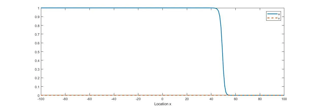
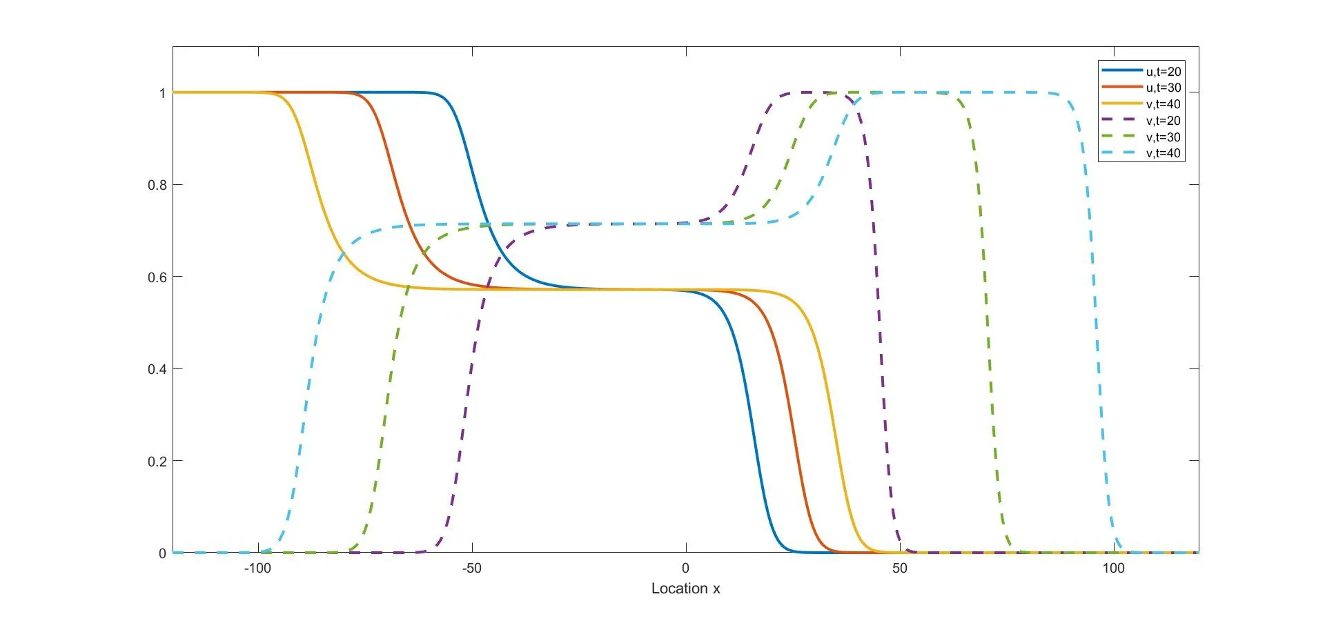
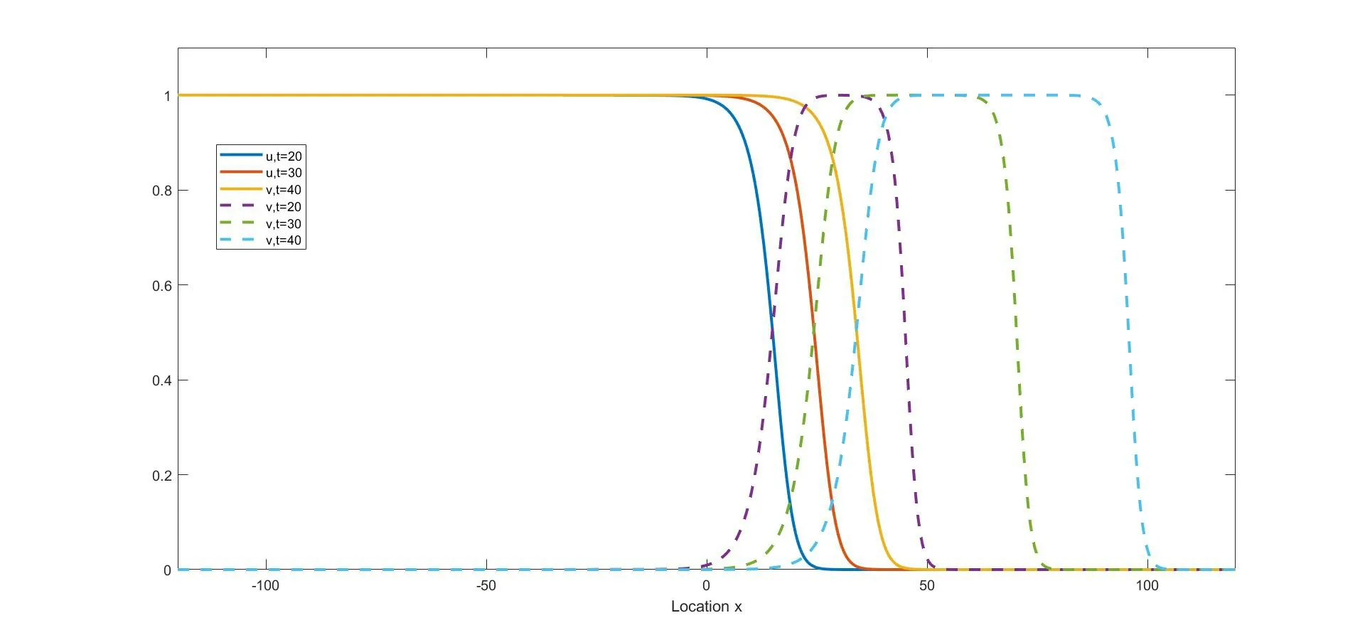
(i) if 0

(ii) if 0

(iii) if 0

(iv) ifa,b>1,then (u(t),v(t)) converges to one of the equilibria u1and u2depending on the initial data (strong competition).

For when the movements of the two competing species happen only between adjacent spatial locations,the following reaction-diffusion Lotka-Volterra competition system,as a counterpart of (1.1),has been widely studied:

We refer to [5,16,26,35,49]for the stability of the steady states u∗,u1,and u2in (1.2).

We consider the wave propagation phenomena of (1.1),which include the studies of traveling wave solutions,entire solutions,and spreading speeds.The traveling wave solution describes the propagation mode of the two competing species,which connects one equilibrium to another equilibrium.We recall some results about the traveling wave solutions of (1.1).The function(u,v)(x,t)=(ϕc,ψc)(ξ) (ξ=x-ct) is called a traveling wave solution of (1.1) with a speedc ∈R if it satisfies that

The existence of positive solutions to(1.3)depends on the parametersaandband the following asymptotic boundary conditions:

(i) when 0

and also admits a positive solution satisfying that (ϕc,ψc)(-∞)=u∗and (ϕc,ψc)(+∞)=u2for each speed

(see Houet al.[25]);

(ii) when 0

(iii) similarly to(ii),when 0

(iv) whena,b>1,system (1.3) admits a unique positive solution satisfying that (ϕc,ψc)(-∞)=u2and (ϕc,ψc)(+∞)=u1with the unique speedc=Cuv ∈R (see Zhang and Zhao[51]).

We refer to [1,7,11,19,53]for more works about traveling wave solutions for (1.1) and[13,23,24]for (1.2).

The entire solution,(which means the solution defined for allx ∈R andt ∈R) is another important research topic.The study of entire solutions can be traced back to the pioneering work of Hamel and Nadirashvili [20,21],in which the authors constructed entire solutions for classical KPP equations in the one-dimensional and high-dimensional spaces by considering the interaction of traveling wave solutions.Since then,many efforts have been made to construct entire solutions of various types;these include the annihilating-front type,which behaves as two opposite wave fronts with positive speed(s) approaching each other from both sides of the real axis and then annihilating as time increases (see e.g.[4,17,31,48]);the merging-front type,which behaves as two monostable fronts approaching each other from both side of the real axis and merging and converging to a bistable front or behaves as a monostable front merging with a bistable front and one chases another from the same side of the real axis (see e.g.[37,47]);the catching-up/invading type,which behaves ast →-∞,like two monostable/bistable fronts moving in the same direction,the faster one then invading the slower one ast →+∞(see,e.g.[22,42]).

In (1.1),different types of entire solutions can provide different propagation and invasion modes of the competing species.For the case 01,Zhanget al.[50]showed the existence of traveling wave solutions and the asymptotic behavior of traveling wave solutions at infinity.For the system (1.2),Duet al.[8,9]studied front-like entire solutions in a periodic habitat.Guo and Wu [18]constructed some new entire solutions which behave as two traveling wave fronts moving towards each other from both sides of thex-axis for discrete diffusive equations.Morita and Tachibana [38]proved the existence of an entire solution which behaves as two monotone waves propagating from both sides of thex-axis.Wanget al.[45]considered the entire solution,which behaves as two wave fronts coming from both sides of thex-axis,for a diffusive and the competitive Lotka-Volterra type system with nonlocal delays.In particular,a new type of entire solution of (1.2),which is different from the aforementioned results,was constructed recently by Lamet al.[29].They showed the existence of entire solutions which asymptotically converge,ast →-∞,to a traveling wave solution consisting of a single species of (1.2) for both the weak and the strong competition cases.Moreover,these entire solutions evolve to distinctive diverging front,whose profiles ast →+∞rely heavily on the competency of each species.

In this paper,we are interested in whether or not the new entire solutions constructed in [29]also exist in (1.1),and in what influence the appearance of the nonlocal dispersals operator has on the construction of this type of entire solution.We show the existence of entire solutions of (1.1) corresponding to (φc(ξ),0) att →-∞,where (φc(ξ),0) is the traveling wave solution of (1.1)consisting of a single species.We also describe the asymptotic behavior of these entire solutions ast →+∞.In the study of the entire solutions,the appearance of a nonlocal dispersal(convolution)operator creates many difficulties.For example,nonlocal dispersal leads to the lack of a regularizing effect;this leads us to encounter a lot of difficulties in sense of the calculation process.Concretely,for the classical Lotka-Volterra competition system studied in[29],the authors studied the existence of entire solutions by introducing co-moving frame,and the existence on entire solutions can be resolved by super-and sub-solutions and estimates for parabolic equations,where the super-and sub-solutions were constructed by considering an eigenvalue-problem.However,we cannot use the estimate for parabolic equations,so we give some estimates and use the Lebesgue dominated convergence theorem to overcome this.Additionally,some methods used for the classical system cannot be applied;these include the fact that the existence of a solution to the eigenvalue-problem for a local system can be obtained directly by virtue of the Hille-Yosida Theorem,but we cannot verify that the Hille-Yosida Theorem is suitable for the system we study,since we cannot prove that the linear operator we construct generates an analytic semigroup of contractions onC0(R),due to the addition of a derivative with respect tox.Hence,we utilize the super-and sub-solutions method to resolve this.During this process,we introduce a technical condition (H) to prove Theorem 2.1.We conjecture that the condition (H) may be non-essential,and that it can be removed by constructing other super-and sub-solutions.Meanwhile,there are many difficulties when we consider the asymptotic behavior of entire solutions ast →∞,since the spreading speed of system(1.1),which will help us to obtain asymptotic behavior att →∞,is not solved for cases 0

Finally,we recall some results on the spreading speed of (1.1).For the casea,b>1,the spreading speed of (1.1) was studied by [51].Moreover,the authors of [12]mentioned that ifa<1

The rest of this paper is organized as follows: Section 2 is devoted to the study of an eigenvalue-problem.Then we construct some new types of entire solutions and study their properties in Section 3.Finally,we present some simulations to illustrate the analytical results in Section 4.

2 Eigenvalue Problems

In this section,we consider the eigenvalue problem of the linearized system of (1.3) at(φc,0).Hereφc(x) is the traveling wave solution of

The equation (2.1) is referred to as the nonlocal version of the classical Fisher-KPP equation[14,28].By the work of Carr and Chmaj [2]and Schumacher [41],we know that (2.1) admits a unique (up to translation) traveling wave solutionu(x,t)=φc(x-ct) connecting 1 to 0 with each wave speed

that is,φc(ξ) solves

For eachc>c∗,there exist some constantsα ∈(α(c),min{1,2α(c)}),A0≫1,x0≫0,(c)>0 andA1such that,by a proper translation the wave profile,φcsatisfies that

whereα(c) and(c) are the smallest positive solutions of

respectively;see [6,36].

In what follows,we always assume (K) and thatr>1.Forc ∈[c∗,+∞),define that

Then there exists a uniqueλ0>0 such that

andF(·) is strictly decreasing on (0,λ0) and strictly increasing on (λ0,+∞).We have that

Byr>1 andb>0,the set Ω∗(c) is nonempty.For anyλ ∈Ω∗(c),we denote thatµ≜F(λ)>r(1-b).For anyc ≥c∗,define that

Note that

Then there exists a uniqueγ>0 such that

The following theorem is the main result of this section:

Theorem 2.1Let (K) and (H) hold.For anyc ∈[c∗,+∞) andλ ∈Ω∗(c),we denote thatµ≜F(λ).Then there exists a solutionwithϕ,ψ ∈C1(R)∩L∞(R) of the following system:

Furthermore,if there existsM<0 such that

then we have that

In order to obtain Theorem 2.1,we first prove the following two lemmas about the existence ofψsatisfying (2.6):

Lemma 2.2Under the same assumptions of Theorem 2.1,there existsψ ∈C1(R)∩L∞(R)satisfying that

whereL>0,λ′∈(λ,min{λ0,λ+α(c)}) withF(λ′)

ProofFor anyλ′∈(λ,min{λ0,λ+α(c)}),the strictly decreasing property ofF(·) on(0,λ0) implies thatF(λ′)

Now we construct a super-solution.For anyβ ∈(0,γ),it follows from(2.5)thatG(β)<µ.Byφc(-∞)=1,we can find a constant∈R small enough such that

Define that

This completes the proof.

Next we recall an important tool called Ikehara’s theorem,whose proof can be found in[10,46].

Theorem 2.3(Ikehara’s) Letwithz ∈C,whereϕ(·)is a positive increasing function on R-.For some real number Λ>0,assume thatP(z) can be written as

wherek>-1,and there is a positive numberεsuch thatQ(z) is analytic in the strip Λ-ε

By Ikehara’s theorem,we can give a more accurate description of the decaying behavior of the solutionψof (2.9) asx →-∞.

Lemma 2.4If there existsM<0 such that

where the functionψis given in Lemma 2.2,then we have that

ProofWe first prove that the equationG(z)=µwithz ∈C has no root exceptz=γin the strip 0

IfG(z)=µ,then

Whenp=γ,byG(γ)=µand the first equation of (2.10),we get that

which implies thatq=0.Whenp ∈(0,γ),by (2.5),we have that

HenceG(z)=µhas no root exceptz=γin the strip 0

Multiplying (2.9) by e-zxand integrating it over R,we obtain that

We have that

which implies that

Define that

It follows from (2.5) that

Theng(·) is continuous on (0,γ].In the strip 0

and it holds that

ThusQ(z) is analytic in the strip 0

which is essentially equivalent to the case whereψ′/ψ ≥Mfor allx<0.This completes the proof.

Now we are ready to prove Theorem 2.1.

Proof of Theorem 2.1By Lemmas 2.2 and 2.4,we only need to prove the existence ofϕ(x).Byψ(x)∈L∞(R) in Lemma 2.2,there existsZ>0 such thatψ(x)≤Z.Define

whereA ≥a/2 andB>aZ/(µ-1).Clearly,(x) is a super-solution of the first equation of (2.6).We next verify thatis a sub-solution of the first equation of (2.6).Whenx≥-λ-1ln(B/A),we have that(x)=-Ae-λx,which,along withψ(x)≤e-λxand (H),implies that

Whenx≤-λ-1ln(B/A),we can get that(x)=-Band

By the standard method of super-and sub-solutions,there is a solutionϕ<0 of the first equation of (2.6) satisfying thatϕ(∞)=0.This completes the proof.

3 Entire Solutions

In this section,we construct some entire solutions of (1.1) and study some qualitative properties of them.We first introduce some notations.For anyc ≥c∗andλ ∈Ω∗(c),denote thatµ≜F(λ),and let (ϕ,ψ) be the solution of (2.6) obtained in Theorem 2.1.For simplicity,we rewrite (1.1) as

where u=(u,v) and

We introduce two increasing functions,p(t) andq(t),satisfying that

whereEis an arbitrary positive constant andω ∈(0,µ/E).Some calculations imply that

It follows that

Define that

It is easy to check thatCλ>Cuv,whereCuvis the unique speed that admits the traveling wave solution connecting u1and u2.Moreover,for eachc ≥c∗,since-cλ+r>0,∀λ ∈Ω∗(c),it follows thatCλ>c.The next two theorems are the main results in this paper.

Theorem 3.1Suppose that (K) and (H) hold.Letc ≥c∗andλ ∈Ω∗(c).Then there exists a unique entire solution uc,λ(x,t)=(uc,λ(x,t),vc,λ(x,t)) of (1.1) satisfying that

Furthermore,for anyν ∈R{0},there exist two positive constantsandsuch that,for any(x,t)∈R2,uc,λ(x,t) satisfies that

Theorem 3.2Suppose that all of the assumptions in Theorem 3.1 hold.Let uc,λ≜(uc,λ(x,t),vc,λ(x,t)) be the entire solution of (1.1) obtained in Theorem 3.1.Then

Furthermore,we have the following statements,which imply that,ast →+∞,the asymptotic behavior of the entire solution depends essentially on the competitiveness of the two species,i.e.,the range ofaandb:

(i) if 0c>C2∗>-C1∗and it holds that

(ii) if 0c>C2∗and it holds that

(iii) ifa,b>1,then there existsξ1∈R such that

where uuv=(ϕuv,ψuv) is the traveling wave solution connecting u1at-∞to u2at +∞,with speedCuv.Furthermore,it holds that

Remark 3.3Notice that the conclusions (3.14) and (3.18) in Theorem 3.2 are obtained onx ∈[(c+∊)t,(Cλ-∊)t]ast →+∞.Actually,we expect that (3.14) and (3.18) hold onx ∈[(C2∗+∊)t,(Cλ-∊)t]ast →+∞,but this is challenging,and fails,sinceC2∗is the minimal wave speed of the traveling waves of the corresponding linearized system (1.1) at (0,1).A classical way of constructing the super-solution of(1.1)iswhenx-ct>0 for some appropriateb,c>0.However,the initial functionvc,λ(x,0) is essentially compactly supported,which does not satisfy that(x,0)≤vc,λ(x,0)whenxis large enough.Hence,we usein (3.8) as a super-solution;this method makes us only prove that uc,λ(x,t) converges to u2forx ∈[(c+∊)t,(Cλ-∊)t]ast →+∞.It is not clear whether or not uc,λ(x,t) converges to u2forx ∈[(C2∗+∊)t,(c+∊)t) ast →+∞;we will leave this for now and hope to solve it later.

For the rest of this section,we focus on the proofs of Theorems 3.1 and 3.2.We first recall the definitions of sub-/super-solutions and the comparison principle of (1.1);see[51,Definition 4.6 and Lemma 4.8].In the next Definition,the definitions of sub-/super-solutions in the weak sense mean that sub-/super-solutions satisfy the integral-differential inequality for all but finite manyt ∈R.

Definition 3.4Let u(x,t)=(u(x,t),v(x,t)) be a piecewise smooth function on R×I,whereI ⊆R is an open interval.Then,

(i) the function u(x,t)=(u(x,t),v(x,t)) is called a sub-solution of (1.1) on R×Iif

(ii) the function u(x,t)=(u(x,t),v(x,t)) is called a super-solution of (1.1) on R×Iif

The following lemma states that,defined by (3.7) and (3.8),are,respectively,sub-and super-solutions of (1.1):

Lemma 3.6Suppose that all the assumptions in Theorem 2.1 hold.Then,forE>max{‖ϕ+aψ‖∞,r‖bϕ+ψ‖∞} and 0<ω<,we have that

ProofBy (2.2),(2.6) and (3.1),we have that,for any (x,t)∈R×(-∞,0],

Similarly,by (2.6) and (3.1),some calculations imply that

Note thatϕ<0<ψ,as stated in Theorem 2.1.By (3.5) and the definitions ofandin (3.8) and (3.7),the proof of (ii) is obvious.

This completes the proof.

The following lemma is a direct consequence of Proposition 3.5 and Lemma 3.6:

Lemma 3.7For anyn ∈Z+,x ∈R andt ∈[-n,0],we have that

In particular,whent=0,it follows that

Now define that

By (3.24),we obtain un(x,t),which,together with the definition of(x,t),yields thatun(x,t)≤1,and there is a constantϑ>0 such that

For any givent∗∈(-∞,0],there existsn ∈Z+such thatt∗>-nand

whereh1=1+aϑ,h2=d+rϑ+rb,and

Then it follows that

The following lemma states some properties about the Lipschitz continuity of(un(x,t),vn(x,t))with respect tox,and the purpose of this lemma is to prove (3.11):

Lemma 3.8Let (K) hold.There is a positive constant,which is independent ofn,xandt,such that,for any (x,t)∈R×(-n,0],

In addition,if(H)holds,then,for anyν ∈R{0}and(x+ν,t),(x,t)∈Ω⊂R×(-n,0],whereΩ is any compact set,there are some constantsN0andindependent ofn,t,andνsuch that

ProofSinceun(x,t)≤1 andvn(x,t)≤ϑ,we can get from (3.28) that,for (x,t)∈R×(-n,0],

By a similar argument as to that for (un)tand (vn)t,we have that

Then (3.32) is proved by taking that

Now,we prove(3.33)and(3.34)on an arbitrary compact set Ω.For anyν ∈R,define that

By the assumptions ofk(x),we have that K′(x)∈L1.Then there is a positive constantKsuch that

Denote that U(x,t)=(U(x,t),V(x,t))=un(x+ν,t)-un(x,t).In order to prove (3.33),we only need to show that

and

Now consider the case in which U(x,t)≥0.Noting that(·,-n)∈C1(R×(-n,0]),there exists a constantM>0 such that

From the first equation of (3.28),we have that

whereM>0 is defined as in (3.35).Then,fort ∈(-n,0],there existsN1>0 such that

SinceUsatisfies that

by the comparison method of ODE,we have that,forx ∈R andt ∈(-n,0],

which implies that

From the second equation of (3.28) and (H),it follows that

Then,fort ∈(-n,0],there existsN2>0 such that

SinceVsatisfies that

by using the comparison method of ODE again,we obtain that,forx ∈R andt ∈(-n,0],

which implies that

For the case where U(x,t)≤0,the proof of U(x,t)≥-N0|ν| is similar.Then (3.33) is proven by taking thatN0=max{N1,N2}.

Forx ∈R,t ∈(-n,0]andν ∈R{0},we can get that

Then we obtain (3.34) by taking thatwhich completes the proof.

Define that

It follows from (3.2) and (3.3) that

We prove the uniqueness of the entire solution satisfying (3.10) by showing that the pair of super-and sub-solutions are deterministic via translation,where the definition is given in [4,Definition 1].Suppose that uc,λ,i(x,t)=(uc,λ,i(x,t),vc,λ,i(x,t)) withi=1,2 are two solutions of (1.1) satisfying (3.10).Then,for anyn ≥|t| and (x,t)∈R×R,we have that

According to (3.8),(3.7),(3.36) and (3.10),we can obtain that

Fori,j ∈{1,2},it follows from (3.36) that

Asn →∞,we get from (3.36) that

which implies that uc,λ,1(x,t)=uc,λ,2(x,t),∀(x,t)∈R2.

According to Lemma 3.8,by the Arzela-Ascoli Theorem and a diagonal extraction process,there exists a function (uc,λ+(x,t),vc,λ+(x,t)) and a subsequence (uni(x,t),vni(x,t)) of(un(x,t),vn(x,t)) such that

converge uniformly in any compact set Ω∈R2to

By the uniqueness of the limit,we have that

Hence,it holds that

The second inequality in (3.11) can be obtained similarly,so the proof is completed.

In order to prove Theorem 3.2,we need to study the asymptotic behavior at infinity of the entire solution uc,λ=(uc,λ,vc,λ) of system (1.1).Notice that the asymptotic behavior of uc,λatt →-∞is a direct result of (3.10).Then we show the asymptotic behavior of uc,λatt →+∞.

Lemma 3.9It holds that

ProofRecall the definition of(x,t) in(3.8).We know that the upper bound in(3.10)holds for allt ∈R;that is,

Therefore,for each∊>0,

On the other hand,the proof of Lemma 2.2 indicates thatψ(x)≤e-λxfor anyx ∈R.Combined with the definition of(x,t) in (3.7),there exists a constantE1>1 such that

Note that e-λ(x-Cλt) andvc,λ(x,t) are a pair of super-and sub-solutions of the following Fisher-KPP equation:

Then the comparison principle yields that

Thus,(3.39) and (3.40) imply (3.37),which completes the proof.

Lemma 3.10It holds that

ProofLemma 3.9 implies that,for any∊>0,

It remains to show that

Similarly to [51,Proposition 4.13],we can prove that

The proof of (3.42) is a straightforward consequence of (3.43).Indeed,if (3.42) is not true,we can suppose,to the contrary,that there exist sequences (tn)n∈N,(xn)n∈Nsatisfying that(c+∊)tn

Lemma 3.11Assuming that 0

ProofFromb<1 anda<1,it follows thatC1∗>0 andC2∗>0,which implies thatC2∗>-C1∗.

We only provide a detailed proof for(ii),since(i)and(iii)can be proven by similar methods.Suppose,by contradiction,that (ii) is false.Then there exists (xn,tn) satisfying that

with initial data (U(0),V(0))=(θ,ϑ),so that (U,V)(∞)=(u∗,v∗).For eachT>0,we have thatand then the comparison in the time interval [-T,0]yields that

In particular,for everyT>0,(,)(0,0)(U,V)(T).LettingT → ∞,we have thatThen it holds that

This is a contradiction,so (ii) is proven.

Finally,we are ready to prove Theorem 3.2.

Proof of Theorem 3.2Note that (3.12) is a direct consequence of (3.10).Now we prove the asymptotic behavior of uc,λast →+∞.

(i) According to the definitions ofCλ,c∗,C2∗,we have thatCλ>c ≥c∗>C2∗.Also,the definitions ofC1∗,C2∗anda,b<1 imply thatC2∗,C1∗>0,and thusCλ>c>C2∗>-C1∗.Furthermore,the conclusion ofc

Next,we prove that

It is clear thatvc,λ(x,t) andϖform a pair of super-and sub-solutions of the equation

withvc,λ(x,t)≥ϖon the boundary of the domain

Then the maximum principle implies thatvc,λ ≥ϖin Ω.Thus,(3.44) holds.

Analogously,we can get that

Naturally,

which,along with (3.45),implies (3.19),by Lemma 3.11 (iii).

(iii) Letξ1∈R,s1,s2,ϱ ∈R+,and define thatThen,similarly to [51,Lemmas 4.16 and 4.19],we can construct a pair of super-and sub-solutions

of (1.1)to prove(3.20).Furthermore,(3.21)–(3.23)follows from[51,Theorem 4.10].The proof is complete.

4 The Exponential Decay Estimates of the Entire Solutions

In this section,we state the exponential decay estimates ofuc,λatx=+∞under the conditions that

Theorem 4.1Letc ≥c∗andλ ∈Ω∗(c).Then we have that

whereα(c) is the smallest positive root of the equationFurthermore,whenb ∈(0,1),we have that

whereγsatisfies (2.5) andNis the constant given by Theorem 2.1.

ProofFrom (3.10),we obtain that

whereψis given by Theorem 2.1.Then (4.2) follows from (2.3),(4.4) and

Since the proof of (4.3) is similar to that of (4.1),we can now prove (4.1) by considering only the following two claims:

Claim 1If there isω0>0 andt0∈R such thatvc,λ(x+Cλt0,t0)≤ω0e-λxforx ∈R,then

Obviously,vc,λ(x+Cλt,t) andω0e-λxform a pair of sub-and super-solutions of the equation

As a consequence,Claim 1 is true.

Claim 2If there existsλ′∈(λ,min{α(c)+λ,λ0}),t0∈R,B0>0 andω0>0 such that

then there existsB1∈(B0,∞) such that

By the second equation of (1.1)anduc,λ(x+Cλt,t)≤φc(x+(Cλ-c)t)≤min{1,e-α(c)(x+(Cλ-c)t)},it can be proven thatvc,λ(x+Cλt,t) is a super-solution of

On the other hand,using a similar argument to that of the proof of Lemma 2.2,we can show that max{0,ω0(e-λx-B1e-λ′x)} is a sub-solution of (4.6),provided thatB1≫B0.Then Claim 2 is obtained.

In virtue of Lemma 2.2 and (4.5),there isB0>0 such that,for any (x,)∈R×R-,

Furthermore,combining this with Claims 1 and 2,we can obtain that,for any<0,there existssuch that

Similarly,one can obtain (4.3).The proof is complete.

Remark 4.2Note that the assumptionis reasonable.Indeed,sinceφc(x)→0 andψ(x)→0 asx →+∞,then,whenx →+∞,the first equation of (2.6)which is satisfied byϕ(x) becomes

Letϕ=-e-δxfor someδ>0.Thenδsatisfies thatNote thatα(c) is the smallest positive solution of

and due toT(0)=1<µ,it follows thatδ>α(c).This,together withyields thatFurthermore,note that the exponential decay estimate ofuc,λwas obtained only atx=+∞(it was absent atx=-∞).The primary reason for this is that the exponential decay estimate ofuc,λwas proven by virtue of (4.4),but the decay estimate of functionϕin (4.4) is not clear atx=-∞,hence we leave this for the further study.

5 Numeric Simulations

We present some numeric simulation results for system (1.1) to demonstrate our analytic.To be computable,we choose the following kernel:

Next,we give a visual description on the behavior of the entire solutions ast →±∞.According to Theorem 3.2,the entire solutions behave like (φc,0) ast →-∞;see Figure 1.

Figure 1 The behavior of entire solutions as t →-∞

Choosea=0.6,b=0.5,d=2 andr=1.7,and clearly 0

According to Theorem 3.2 (i),the two species invade (1,0) from (u∗,v∗) to the left ofxwith speed-Cλ,invade (0,1) from (u∗,v∗) to the right ofxwith speedC2∗

Figure 2 The profiles of (u,v) at t=20,30,40 in the case where 0

Choosea=0.6,b=1.2,d=2 andr=1.7,and clearly 0

Figure 3 The profiles of (u,v) at t=20,30,40 in the case where 0

Choosea=1.1,b=1.2,d=2.3 andr=2.2,and clearlya,b>1,we have that

By Theorem 3.2 (iii),the two species invade (0,1) from (1,0) to the right ofxwith speedCuv,invade (0,0) from (0,1) to the right ofxwith speedCλ,and finally,the long-time behavior of the entire solutions ast →∞is described by (3.20)–(3.23);see Figure 4 for details.

Figure 4 The profiles of (u,v) at t=15,30,45 in the case where a,b>1

Conflict of InterestThe authors declare no conflict of interest.