Displacement-based back analysis of mitigating the effects of displacement loss in underground engineering

Hui Li, Weizhong Chen, Xianjun Tan

State Key Laboratory of Geomechanics and Geotechnical Engineering, Institute of Rock and Soil Mechanics, Chinese Academy of Sciences, Wuhan, 430071, China

Keywords:

ABSTRACT Displacement-monitoring-based back analysis is a popular method for geomechanical parameter estimation.However, due to the delayed installation of multi-point extensometers, the monitoring curve is only a part of the overall one, leading to displacement loss.Besides, the monitoring and construction time on the monitoring curve is difficult to determine.In the literature, the final displacement was selected for the back analysis,which could induce unreliable results.In this paper,a displacement-based back analysis method to mitigate the influence of displacement loss is developed.A robust hybrid optimization algorithm is proposed as a substitute for time-consuming numerical simulation.It integrates the strengths of the nonlinear mapping and prediction capability of the support vector machine(SVM) algorithm, the global searching and optimization characteristics of the optimized particle swarm optimization (OPSO) algorithm, and the nonlinear numerical simulation capability of ABAQUS.To avoid being trapped in the local optimum and to improve the efficiency of optimization, the standard PSO algorithm is improved and is compared with other three algorithms (genetic algorithm (GA), simulated annealing (SA), and standard PSO).The results indicate the superiority of OPSO algorithm.Finally, the hybrid optimization algorithm is applied to an engineering project.The back-analyzed parameters are submitted to numerical analysis, and comparison between the calculated and monitoring displacement curve shows that this hybrid algorithm can offer a reasonable reference for geomechanical parameters estimation.

1.Introduction

In the process of underground excavation, it is critical to determine in situ stress and properties of rock masses.Unreliable parameters used for stability analysis may lead to unreliable judgement, then, threaten human safety and property.Conventional methods for parameter estimation are focused on the field or laboratory experiments, which are time-consuming, uneconomic,and unrepresentative for the reason of limited sampling.

The displacements recorded and enriched during the excavation process are generally deformations of the surrounding rocks under the specific excavation schemes.Therefore, the displacements are regarded as the most common indictor to perform a retroactive analysis of geomechanical parameters.Generally, the methods of back analysis include three categories (Qi and Fourie, 2018),including analytical or semi-analytical methods (Feng et al.,1999;Bertuzzi,2017),numerical analysis(Hisatake and Hieda,2008;Luo et al., 2018), and intelligent back analysis (Hashash et al., 2010;Miranda et al., 2011; Gao and Ge, 2016; Liu and Liu, 2019; Zhang et al., 2020a, 2020b).For analytical or semi-analytical methods,there are various assumptions and simplifications, which is unsuitable for complex geotechnical engineering (Zhao and Feng,2021).It is convenient to adjust models and calculation conditions, and obtain different types of results at a time by numerical analysis.The back analysis by numerical analysis is based on trialand-error or gradient optimization method (Khamesi et al., 2015;Manzanal et al.,2016).However,it needs repetitive calculations in practical engineering.

The swift progress in computer science and artificial intelligence has led to the extensive utilization of artificial intelligent optimization techniques in geotechnical engineering to back analyze geomechanical parameters(Miranda et al.,2011;Kang et al.,2017),rheological parameters (Qi and Fourie, 2018), seepage parameters(Wu et al.,2019), parameters about constitution model (Gao et al.,2020), and in situ stress (Bertuzzi, 2017).The intelligent datadriven algorithms consist of Gaussion process (GP), artificial neural network (ANN), support vector machine (SVM), random forest(RF), extreme learning machine (ELM), and improved algorithms optimized by particle swarm optimization(PSO)algorithm,genetic algorithm(GA),ant colony optimization(ACO),and Jaya algorithm(Drucker et al., 1997; Jiang et al., 2018; Thang et al., 2018; Al-Thanoon et al., 2019; Zhang et al., 2019; Huang et al., 2020a, b, c;Chang et al.,2020).They are constructed for mapping the nonlinear relationship of datasets and building a substitute model for numerical analysis by training and evaluation.In other words, the optimization problem involved in the back analysis of geomechanical parameters aims to identify the parameter set that minimizes the difference between the calculated and monitored displacements.In geotechnical engineering,the SVM algorithm is a reliable method for classification, estimation, and pattern recognition(Drucker et al.,1997;Thang et al.,2018).The major advantage of SVM is its capability of solving problems with small datasets(Cao et al., 2016).Nevertheless, the generalization and prediction capability of SVM algorithm are affected by the hyper-parameters.On the other hand,the PSO algorithm is proven to be one of the most useful algorithms for optimizing artificial intelligent model (Al-Thanoon et al., 2019; Tang et al., 2019).Unfortunately, the standard PSO algorithm has the disadvantage of being trapped in the local optimum due to the improper inertia weight and the unicity of searching space.

Furthermore, the selection of calculated data corresponding to monitoring data is of importance, affecting the accuracy of backanalyzed parameters.In numerical analysis, the displacements are recorded upon the layer excavation, indicating the overall deformation caused by disturbance.However, in practical engineering,the multi-point extensometers are always assembled after the preliminary support.The displacement values that occur before the installation of sensors are called displacement loss, which is difficult to determine.In the literature, the displacement loss is considered by introducing the load or displacement release coefficient(Gao and Ge,2016),which is determined by experience and is somewhat unreliable (Lu et al., 2014).Only a direct method to obtain the displacement loss is proposed by applying the Hoek experimental formula and monitoring data (Zhang et al., 2009).Nevertheless, it is raised by the experimental formula of homogeneous and isotropic rock mass, and it is only appropriate for the two-dimensional (2D) planar problem.On the other hand, the deformations of surrounding rocks at various monitoring points vary with the excavation process, resulting in different deformation curves.Therefore, the deformation is the function of the time and location of the monitoring points.In the monitoring curve, the initial monitoring time and construction time are difficult to determine and correlate with the simulation curve.As aforementioned, the key for precisely obtaining the geomechanical parameters is to determine a suitable time corresponding to the monitoring curve.

In this paper, we propose a hybrid displacement-based back analysis to mitigate the influence of displacement loss.To reduce the repetitive numerical analysis, the standard PSO algorithm is first improved, and it is used for the training of SVM model.Then,the optimized PSO algorithm is used to search for the optimal geomechanical parameters.Besides, a data reconstruction method is developed based on the start and end time of the layer excavation of rock mass.The displacement difference in the period of time when considerable displacement occurs is selected to correlate with that in the simulation curve.

2.Methodology

2.1.Mathematical introduction of back analysis method

The process of back analyzing geomechanical parameters is an optimization issue,where the decision variables are the parameters of the surrounding rocks, and the output variables are the displacement responses.The objective is to minimize the sum of squared errors (SSE) between the calculated and monitored displacements, and the optimal solution ensures that the calculated displacements match well with that observed in situ.The fundamental concept of the back analysis involves using an iterative approach to derive a set of geomechanical parameters that can optimize the following optimization objective function.

Assuming that an m-dimensional matrix defined as X contains all parameters to be inversed (see Eq.(1)), and the quantity of monitoring points is assumed as n.Then, the objective function is illustrated in Eq.(2).

where Ψ（X*） is the optimal objective function value, Ψ（X） is the objective function value for X, u*iis the true monitoring displacement of ith point,and ui（X）is the calculated displacement for X of ith point.

Eq.(3) can be used to limit the acceptable range of each geomechanical parameter in practical engineering.The determination of this range can be achieved by conducting laboratory or in situ experiments,or by consulting rock mass classification standards.By doing so, the computational cost can be minimized while improving the accuracy of back analysis.

where ximinand ximaxrepresent the lower and upper bounds of the geomechanical parameters,respectively,which are estimated prior to the back analysis.

2.2.Optimized particle swarm optimization (OPSO) algorithm

The PSO is a stochastic optimization algorithm proposed by Eberhart and Kennedy in 1985 (Kennedy and Eberhart,1995) and inspired by animal social behavior.It has gained popularity due to its simplicity, ease of implementation, and fast computation time.The algorithm initializes each particle with a stochastic position and "fly" velocity, which is updated using Eqs.(4) and (5).During each iteration,the optimal position of all particles and the historical best position of the ith particle are recorded and modified.As the iterations progress, the particles gradually converge towards the global optimal solution (see Fig.1).

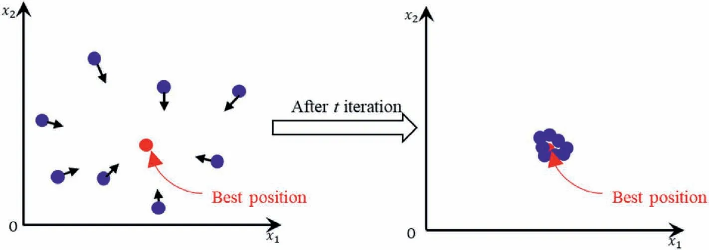
Fig.1.Schematic diagram of particle swarm algorithm (Zhou, 2016).

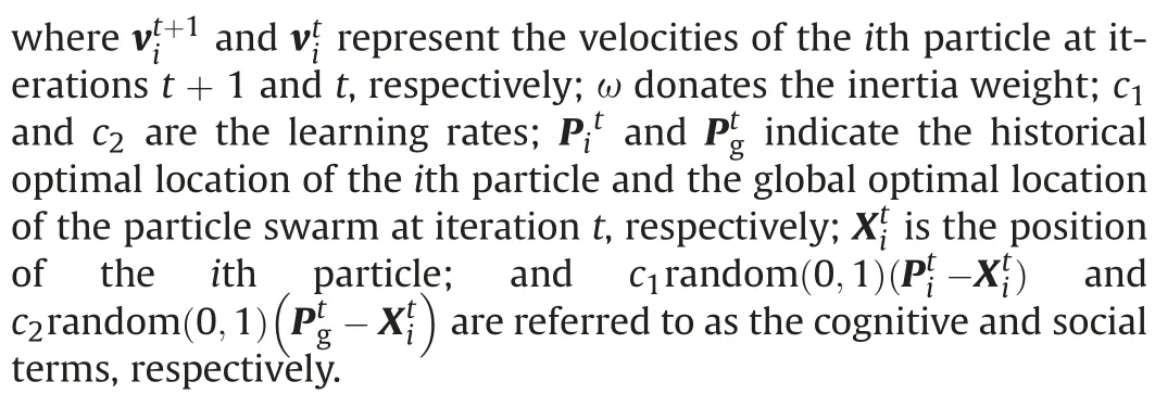
The convergence rate and accuracy of the algorithm can be adjusted by modifying the inertia weight ω, which is a crucial parameter.Previous research shows that increasing the coefficient value enhances the particles’ability to explore and search,thereby increasing the chances of escaping local optima.Conversely,decreasing the coefficient value enables the particles to obtain more precise results (Maliheh et al., 2022).To improve the optimization capability of the algorithm, increasing the inertia weight at the earlier stage and decreasing it at the later stage will lead to a more robust capability for the optimum.Thereafter, a determination method for the inertia weight is proposed by identifying the customized time node︿t,before which the higher value is confined and after which the lower one is assigned compared with the linear function of inertia weight.One can derive the inertia weight estimation by utilizing Eq.(6), and the correlation between the generation and the inertia weight value can be observed in Fig.2:

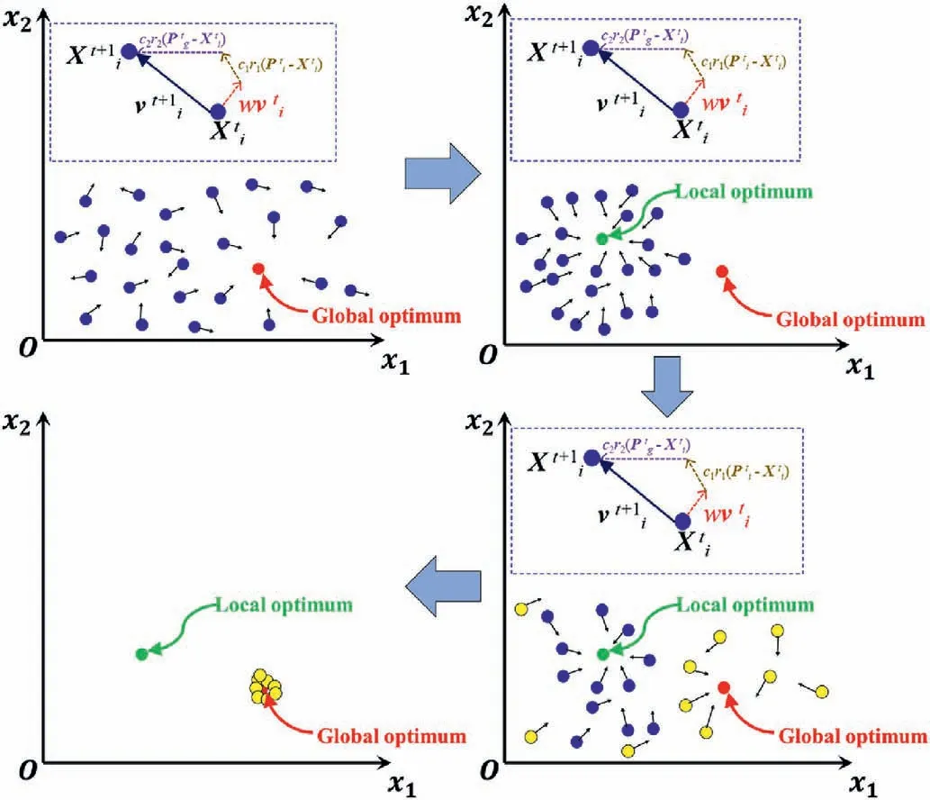
Fig.3.Schematic diagram of particle reset mechanism.

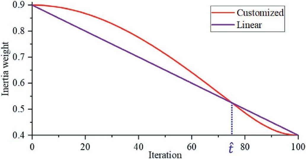
Fig.2.Curves of inertia weight with iterations.

where ωminis the minimum inertia weight,ωmaxis the maximum inertia weight, and tmaxis the total iterations.

On the other hand, the range of search space shrinks with iteration.When particles are trapped in a local optimum, it becomes difficult for them to escape.Therefore, in order to deal with complex nonlinear mapping relationships,it is crucial to enhance both the homogeneity and diversity of the evolutionary population.To achieve this,a particle reset mechanism has been proposed,which randomly reinitializes a certain percentage of particles in the search space during each iteration.In this context,the reset proportion is established as 0.2 and is demonstrated in Fig.3.

To verify the feasibility of the proposed optimization algorithm,it is used in the optimum estimation of four classical functionscompared with the other three widely used optimization algorithms including GA, simulated annealing (SA) algorithm, and standard PSO algorithm.Table 1 presents a list of the expressions,optimums,and searching ranges of the four classical functions,and the graphs of the functions are shown in Fig.4.For simplification,the theories of GA and SA can be detailed in other literature.Besides, the relevant parameters of GA are set as follows: the quantity of initial popular is 30;the crossover probability is 0.5;the mutation probability is 0.4;the selection probability is 0.9,and the maximum number of iteration is 200.The relevant parameters of SA are set as follows:the initial and final temperature are 100 and 0.01, respectively; the cooling speed is 0.9; the maximum number of iterations is 200; the maximum number of attempts in each temperature range is 80.The standard PSO and OPSO algorithm are utilized with the same setting for the common parameters.For instance,the dimensions of the functions are 10,and the quantity of particles is 30,the maximum number of iteration tmax= 200,the learning rates c1= c2= 2, respectively.While for the specific parameters of OPSO, the maximum and minimum of inertia weights are set as: ωmin= 0.4,ωmax= 0.9, the customized time node︿t = 0.75× 200 = 150, and the re-initialization ratio is 0.2.For standard PSO,ω is considered a constant equal to 0.8.

Table 1 Properties of testing functions.

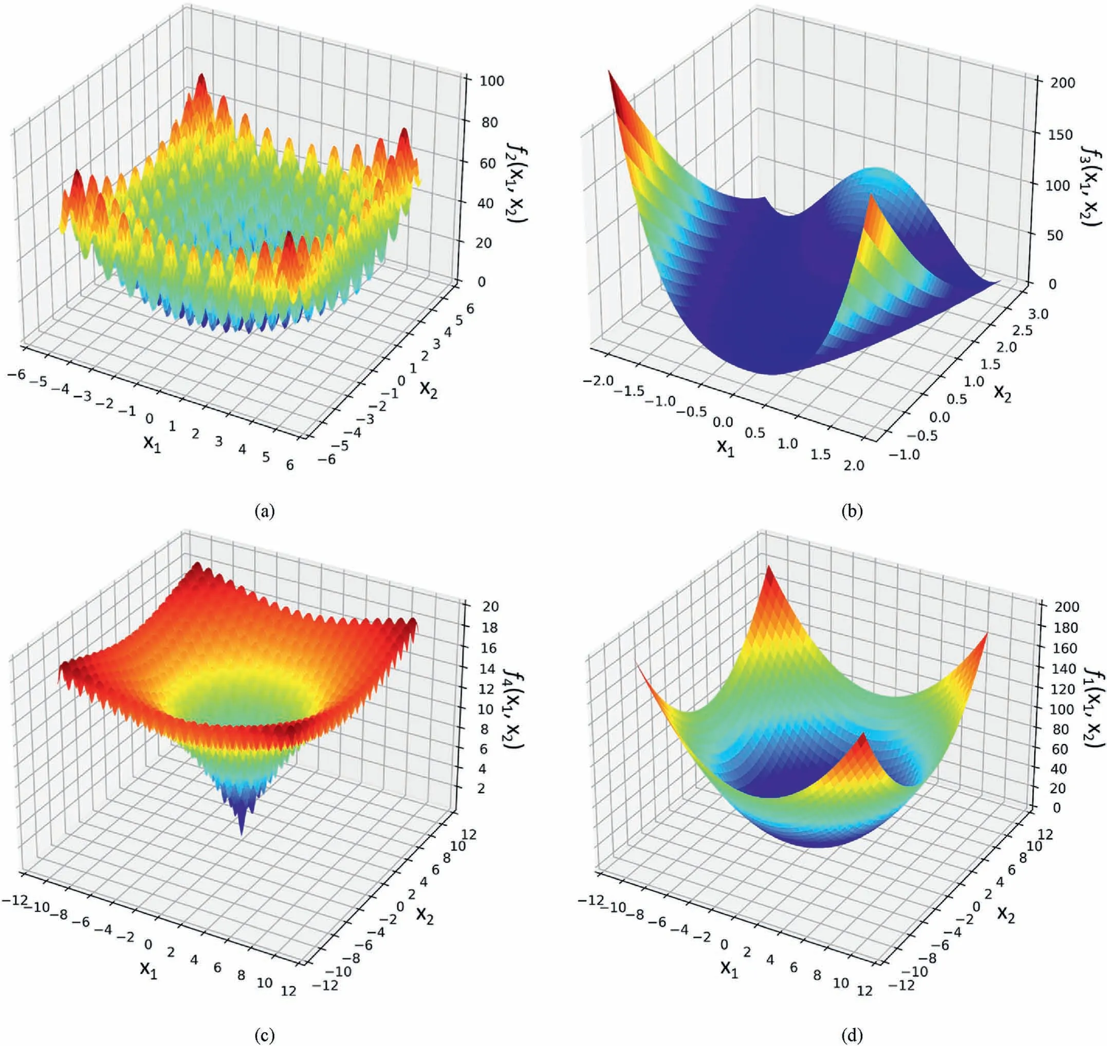
Fig.4.Schematic diagrams of typical testing functions: (a) Rastrigin, (b) Rosenbrock, (c) Ackley, and (d) Sphere.

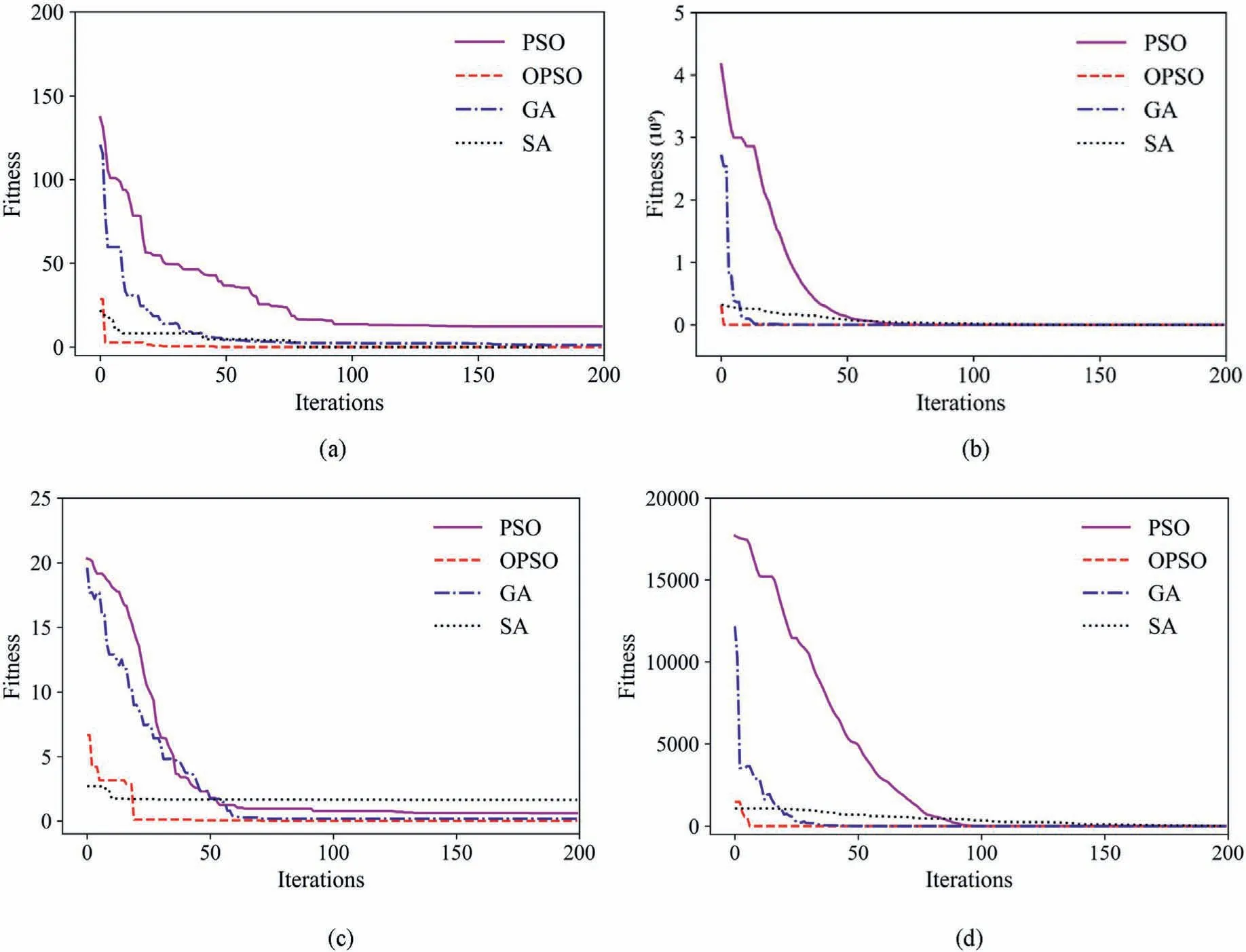
Fig.5.Comparison of the evolution curves for different optimization algorithms: (a) Rastrigin, (b) Rosenbrock, (c) Ackley, and (d) Sphere.

The variation curve of the relationship between fitness and the number of iterations is shown in Fig.5.It can be seen that these fouralgorithms have outstanding optimization capability,by which the final minimums are close to the global optimal values.Nevertheless, the proposed OPSO algorithm outstands from all of the four algorithms in convergence rate and accuracy.Take the Rastrigin function for example,which is a multiple hump function,the result is already close to the global optimal value after 46 iterations,while after 176,177, 78 iterations for PSO, GA, and SA, respectively, with the calculated optimum to be 1.1 × 10-3, 12.3, 1.16, 1.6 × 10-3,respectively.The detailed quantity of convergence iterations and calculated optimal values are listed in Table 2.

2.3.SVM algorithm

The SVMs utilize structural risk minimization to achieve strong generalization capabilities, as noted by Ke et al.(2021).Originally proposed for binary classification problems, SVMs search for the optimal hyperplane.However, for complex datasets, the hyperplane in the original space may be nonlinear,necessitating the use of a nonlinear kernel to transfer the data to a higher dimension of the feature space and weaken the nonlinear characteristics of the data (see Fig.6).The "support vectors" are the adjacent points to the hyperplane, and the optimal function of the hyperplane is the one with the maximum margin between the hyperplane and the"support vectors" (Zhou, 2016).Table 3 lists the most commonly used kernel functions.In addition to binary classification problems,Drucker et al.(1997) expanded the application of the SVM algorithm to regression problems, resulting in the development of support vector regression (SVR).

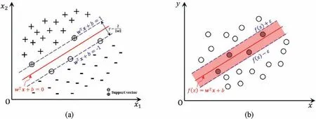
Fig.6.Diagrams of SVMs: (a) support vector classification, and (b) support vector regression (Zhou, 2016).

Table 3 Common kernel functions.

2.4.Comprehensive algorithm for back analysis considering displacement loss and uneven data

The aforementioned theory shows the importance of the parameters in kernel functions.Empirical methodology, cross validation, and grid search cross validation (GridSearchCV) are commonly employed to estimate the hyper-parameters of kernel functions.While, they are no doubt inefficient, imprecise, and uneconomical.With the help of the proposed OPSO algorithm,which is proven to be robust in optimization problem, the optimal parameters of kernel function can be estimated.Therefore,the OPSO algorithm can be utilized for parameter estimation and optimal solution calculation.Besides,for the back analysis of rock mass,the aim is to minimize the fitness function,which is commonly defined as SSE between the actual and predicted displacement.The relationship of the geomechanical parameters with displacement response needs to be trained with datasets,which can be obtained numerically (Reuter et al., 2018), such as ABAQUS.Thereafter, the OPSO-optimized-SVM models are the substitute for displacement prediction.The algorithm that combines the advantages of global search and optimization features of OPSO,the prediction capability of SVM,and the nonlinear numerical analysis function of ABAQUS,is thus named as OPSO-SVM-ABAQUS algorithm.The comprehensive analytical framework is illustrated in Fig.7.The pivotal implementation steps are stated as follows:

(1) Step 1: Estimate inversed parameters of rock mass.The parameters to be back analyzed are generally those that have a great influence on the stability of surrounding rock mass and are difficult to be accurately estimated by experiments.Experimental schemes are constructed using an orthogonal or uniform experimental design.

(2) Step 2: The numerical analysis model and automatic calculation process for various groups of properties are executed for the displacement response at monitoring points.According to the in situ monitoring curve, the period when displacements vary significantly is selected for back analysis.The start time is when the specific layer excavation of rock mass and the end time represents the completion of a layer excavation.The displacement difference during this period is regarded as the output variable for back analysis.Therefore,the input variables are the physical and mechanical parameters of rock mass, and the output values are displacement differences at each monitoring point.

(3) Step 3: The corresponding numerical results need to be reconstructed for the numerical displacement differences and then divided into training and testing datasets by the specified proportion.The normalization pretreatment is carried out to avoid over- or under-fitting.

(4) Step 4: The initial particle swarm is established for SVM variables (the regularization coefficient C, σ2, and the tolerance error ).In this step, the dimension of each particle is three.

(5) Step 5: Because of the special feature of SVM model, the quantity of SVM model is determined by the number of output variables.Considering that the monitoring displacement differences are true values, and the objective is to minimize the root mean squared error(RMSE)of monitoring values and predicted ones.The RMSE is also set to be the fitness of each particle.Simultaneously, the global and particle optimal fitness are recorded.Iterations continue until the convergence condition is satisfied.Before that, the positions and velocities of the particles are updated by Eqs.(4)and (5), and then, the positions of 0.2 particles are reinitialized.Finally, the optimal SVM model is obtained.

(6) Step 6: The initial particle swarms are generated based on the physical and mechanical parameters.In this step, the dimension of each particle is estimated by the quantity of parameters to be inversed.

(7) Step 7: In this step, the SSE of monitoring and predicted displacements is considered to be the fitness function, and the goal is to record the global and particle optimal fitness and corresponding input values.

(8) Step 8: If the convergence condition is not satisfied, update the properties of particles by Eqs.(4) and (5), and then reinitialize the position of 0.2 particles.Repeat steps 7-8 until the termination condition is met.The position of particle with minimum fitness is the optimal solution.

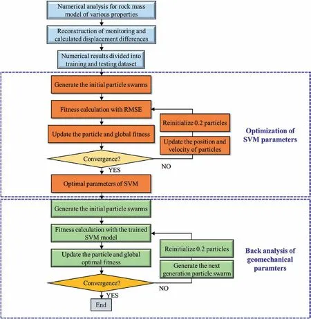
Fig.7.Flow chart of the proposed OPSO-SVM-ABAQUS algorithm.

The key step is to fabricate the dataset,which is the pivotal issue for model training and prediction.The displacement of the surrounding rock mass frequently occurs before sensors are installed;while upon excavation, an amount of energy is released, which occupies the majority proportion, leading to displacement loss.Actually,the calculated displacement represents that for the entire construction process, while the monitoring displacement is only a part of that.In theory, the overall displacement is the sum of monitoring displacement and displacement loss.Besides, considering the different performance of monitoring instruments at the same monitoring section,displacement values need to be aligned in time, and the starting points of valid monitoring values need to correspond to the number of the excavated layers.

3.Case study

To verify the performance of proposed displacement-based back analysis approach, it was applied to the Suki Kinari underground powerhouse caverns.

3.1.Background of Suki Kinari underground powerhouse caverns

The Suki Kinari (SK) hydropower project is situated at the Kunhar River, Khyber Pakhtunkhwa Province.The main powerhouse is buried 450 m vertically, and 250 m horizontally.The section shape is a straight wall with arch roof and the excavation size is 24 m × 53 m × 134.6 m (width × height × length).The width,height, and length for the main transformer chamber is 7.8 m,33.35 m, and 126.85 m, respectively.The inter-distance of them is 45 m.The powerhouse caverns are excavated by the layered excavation scheme.

The regional strata are metamorphic pebbled lithic quartz sandstone (MPLQS), metamorphic sandy Bibbey-rock (MSB), and metamorphic basalt (MB) of Panjal formation.The strike of the foliation is NE60°-80°, with a dip angle of 70°-85°.Three largescale faults develop about 0.8 km near the caverns.The initial geostress conditions are that the maximum horizontal principal stress is 11.1-14.3 MPa with an orientation of NW38°-66°; the minimum horizontal principal stress is 7.5-9.5 MPa, mainly with an orientation of NNW-NWW.The maximum lateral pressure coefficient is 0.9-1.2, with an average of 1.1.Three sections are selected to install multipoint extensometers to monitor the deformation of the surrounding rock mass.The arrangement of multipoint extensometers is shown in Fig.8.

During the construction of underground structures, the displacement monitors are always installed after the completion of the first lining (Zhao and Feng, 2021).The quality of displacement monitors and excavation disturbance affect the displacement records,leading to displacement loss,missing,or abnormity.The actual displacement curves of low quality are illustrated in Fig.9.By analyzing the monitoring displacement data, the displacements at four monitoring points are chosen for the back analysis.The specific locations of the four monitoring points are shown in Fig.10.

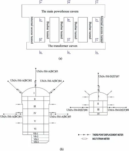
Fig.8.Layout of the monitoring instruments: (a) Location of the typical monitoring cross-sections, and (b) Arrangement of sensors.

The first and essential operation is data construction.To compare monitoring data with numerical values,both of them are required to be reconstructed by setting the displacement at the beginning of one layer excavation to be 0.The displacement difference during the period when the displacement varies with tunnel excavation obviously is selected for back analysis.The displacement at the left sidewall of the main powerhouse is used for the study.The multipoint extensometers were assembled on 28 October 2019,and it is also the excavation time for the fifth layer of the main powerhouse.From the curve of displacement versus time(see Fig.9c),we can know that the displacement at the monitoring point becomes stable until 9 February 2020, which is also the completion time for the excavation of the sixth layer of rock mass.Therefore,the end time node of data used for back analysis is set as 9 February 2020.During 28 October 2019 to 9 February 2020, the displacement difference is calculated as 28.3 mm, which is regarded as the actual displacement difference.In this way, we replace the overall displacement with relative displacement difference,which mitigates the influence of displacement loss and low quality of monitoring data.Correspondingly,we recode the numerical data in the same way.

3.2.Results and discussions

Obtaining the geomechanical parameters necessary for inversion through experiments is a challenging issue.Nevertheless,they are essential for maintaining the stability of the surrounding rock mass during construction.These parameters include elastic parameters, plasticity, damage parameters, and rheological parameters.To address this, we have selected the elastic modulus and cohesion of three different classes of surrounding rock mass(E1,C1,E2, C2, E3, C3) for back analysis.The searching range of each parameter is exhibited in Table 4.

Forty groups of datasets are constructed by the orthogonal experiment design, including six geomechanical parameters and corresponding displacement differences at four monitoring points.Then,theyarerandomly dividedinto32trainingsetsandeighttesting sets.The former is trained for the nonlinear mapping relationship,while the latter serves as evaluation tools to verify the model’s dependability through RMSE and the determination coefficient(R2):

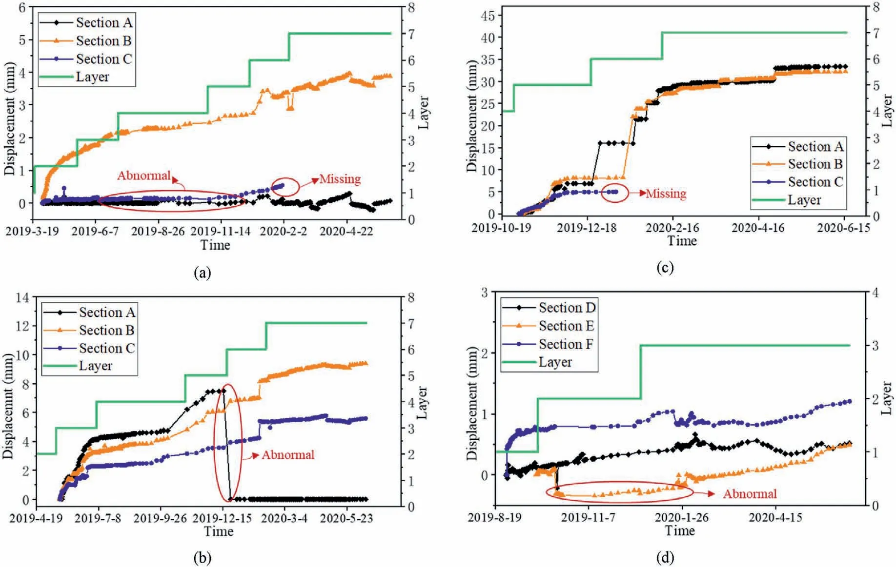
Fig.9.Monitoring curves at key points: (a) the arch vault, (b) the right spandrel and (c) the left sidewall of the main powerhouse, and (d) the arch vault of the transformer powerhouse.

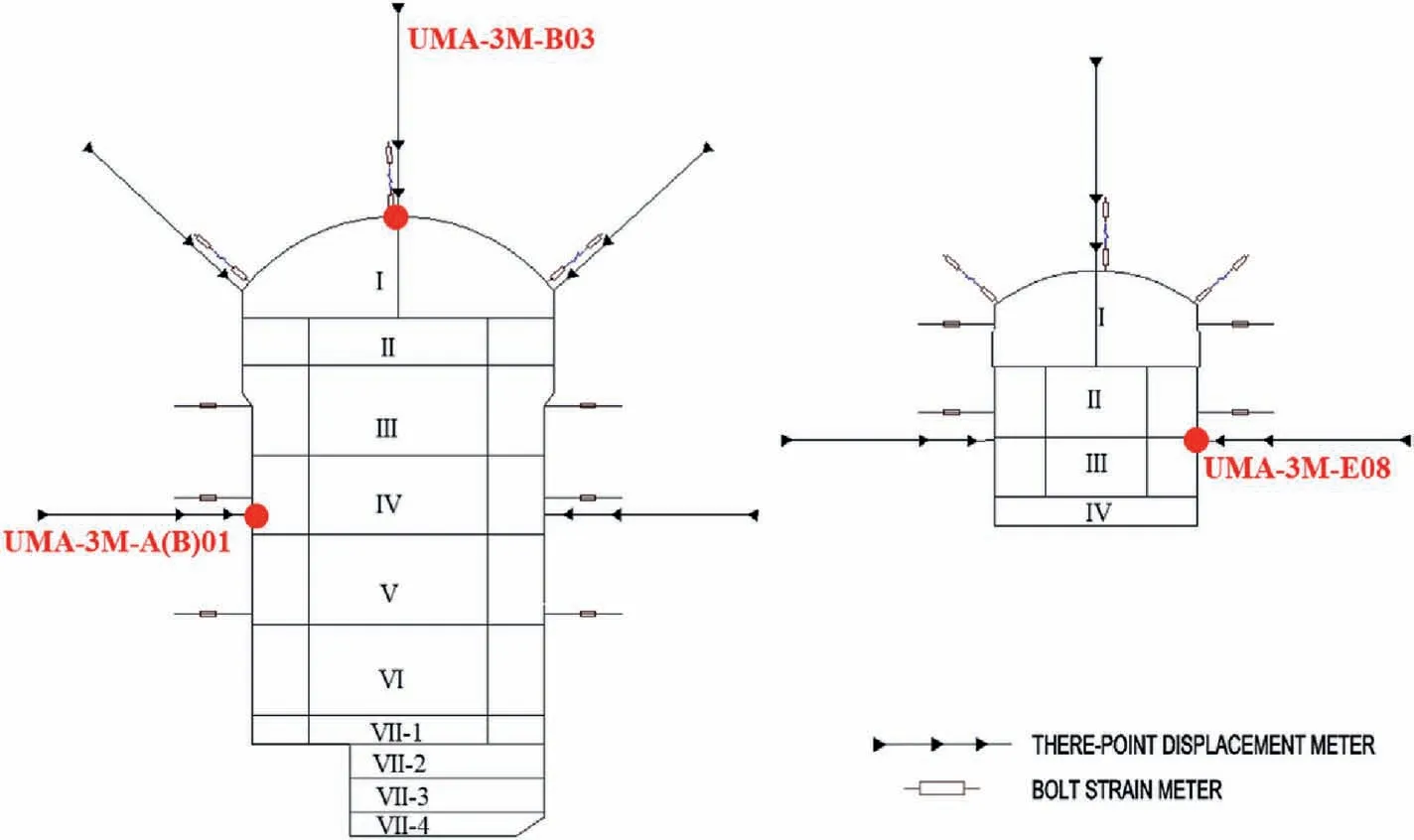
Fig.10.Location of the key points.

where yi,︿yiare the predicted and actual data,respectively;and yiis the mean of actual values.

As aforementioned, the kernel function of SVM affects the generalization capability.Therefore,we examined the effectiveness of the SVM algorithm trained with different kernel functions, and the corresponding evaluation metrics are presented in Figs.11 and 12.It can be seen that the trained SVM model is of the lowest RMSE value and the highest R2value for the radial basis kernel function(RBF),indicating the optimal performance on prediction.To obtain the hyperparameters of the SVM model for the best nonlinear mapping relationship on the geomechanical parameters and displacement differences, the proposed OPSO algorithm is utilizedfor four SVM models.The search for the best parameters of each trained SVM model is conducted within the intervals of C = [0.01,1000],γ = -（2σ2）-1= [0.1,10],and =[10-8,0.1].The searching velocity for each dimension is vC= [- 100,100], v= [- 10-2,10-2],and vγ= [-1,1].The OPSO parameter setting is c1= c2=2, ωmin= 0.4, ωmax= 0.9, tmax= 300, n = 30, ︿t = 0.75×300 = 225, and the re-initialization ratio is set to 0.2.Subsequently, the SVM that has been trained is considered as a replacement for the unnecessary numerical analysis.The objective of the inversion analysis is to identify a group of geomechanical parameters that minimize SSE between the computed and monitored displacements.The searching range and searching velocities of back-analyzed parameters are listed in Table 4.The parameters of OPSO algorithm are set as c1= c2= 2, ω = [0.4,0.9], tmax=1000,n = 100,︿t = 0.75×1000 = 750,and the re-initialization ratio is 0.2.To eliminate the accidental error of calculation,we run five times independently for each method.The average of the backanalyzed parameters is taken as the final geomechanical parameters.The results are tabulated in Table 5.

Table 4 Properties of surrounding rock mass and searching range.

To validate the back-analyzed geomechanical parameters, six key points were chosen for the comparison of displacements obtained by numerical calculation and in situ monitoring.The locations of the key points are indicated in Fig.13.The displacement data monitored and calculated at the monitoring points during the excavation process are depicted in Fig.14.The entire calculated displacements are larger than the monitoring data and the regularity of the calculation curve is consistent with the monitoring curve.Amount of energy releases as soon as the surrounding rock mass is excavated,leading to displacement loss.Numerical analysis has the advantage of recording overall displacements, including displacement before excavation, the one that occurs during excavation and supporting, and that occurs during supporting and installation of multipoint extensometers.Nevertheless, the monitoring curve is merely a part of the displacement curve, recording the displacement which occurs after the installation of monitors.In other words, the calculated displacements are the sum of displacement loss and monitoring displacement.

As a result, the geomechanical parameters obtained through back analysis can effectively reflect the characteristics of the surrounding rock mass, as evidenced by the comparison of displacement monitoring data.The reliable parameters ensure the accuracy of stability analysis, as well as the optimization of excavation and support strategies.

4.Conclusions

A displacement-based back analysis method is proposed accounting for displacement loss.To reduce the repetitive simulation,the advanced SVM model combined with OPSO and ABAQUS is used.Application of an engineering project indicates that the method can offer high precision and a benchmark for back analysis of geomechanical parameters based on the reconstructed monitoring curve.The findings are drawn as follows.

(1) The OPSO algorithm is advanced by enhancing the uniformity and variety of the evolutionary population, as well as defining a modifiable inertia weight.Comparison is implemented for PSO, OPSO, GA and SA from accuracy and efficiency.Results reveal that the OPSO is superior to the other three algorithms.

(2) A hybrid algorithm is presented that integrates the nonlinear mapping and prediction function of SVM, the global searching and optimization features of OPSO, and the nonlinear numerical analysis capability of ABAQUS to leverage their respective strengths.

(3) A data reconstruction method is adopted.Focusing on the period when displacements vary significantly with the excavation scheme, the start time is selected as the beginning of a specific layer excavation, and the end time represents the completion of a layer of the rock mass.The displacement difference during the start and end time corresponds to that of the numerical curve.

(4) The back-analyzed geomechanical parameters for Suki Kinari underground powerhouse caverns are resubmitted to numerical analysis.The results of the calculated curves and monitoring ones demonstrate that the back-analyzed parameters have a high precision.

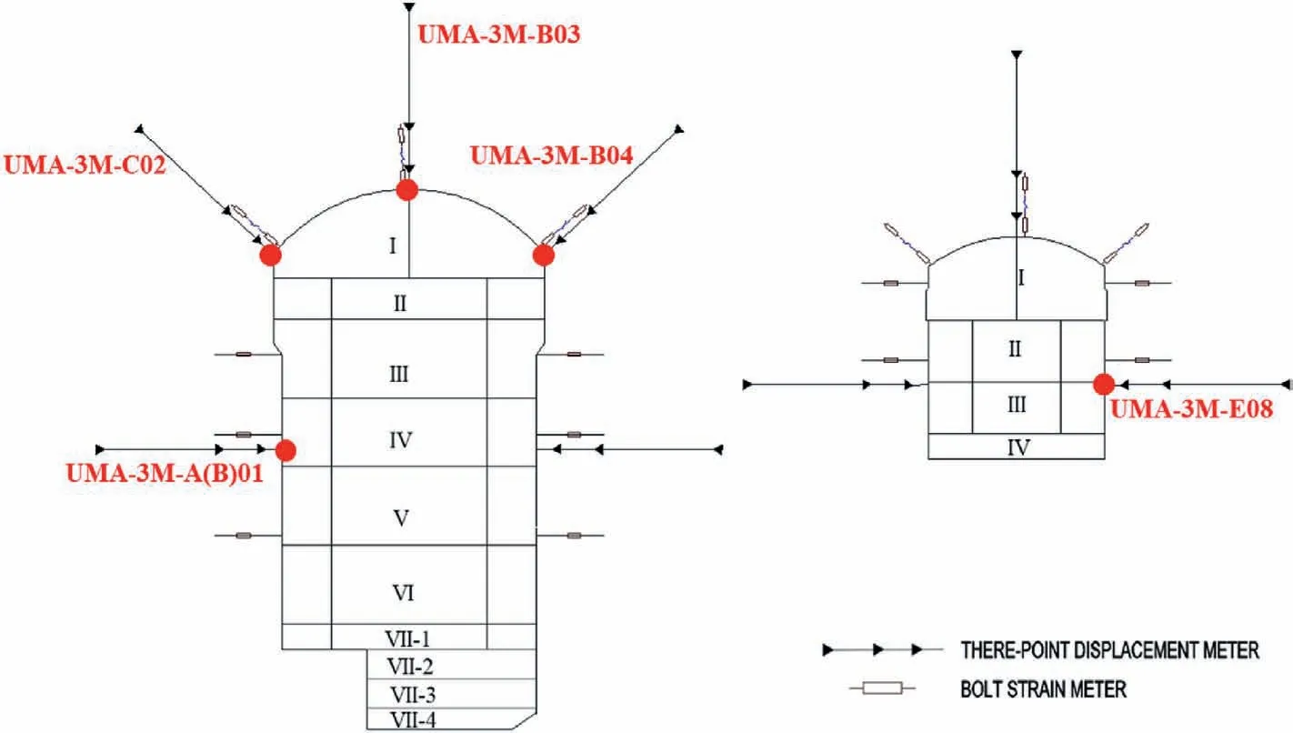
Fig.13.Location of the key points.

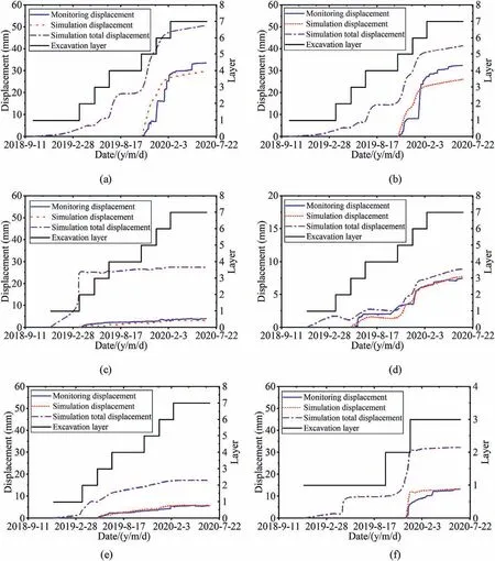
Fig.14.Comparison of the displacement between in situ and calculated results at monitoring points:the left sidewall of the main powerhouse at(a)section A,and(b)section B,(c)the arch vault,and(d)the right spandrel of the main powerhouse at section B,(e)the left spandrel of the main powerhouse at section C,and(f)the right sidewall of the transformer powerhouse at section E.

Declaration of competing interest

The authors declare that they have no known competing financial interests or personal relationships that could have appeared to influence the work reported in this paper.

Acknowledgments

The authors express their gratitude for the assistance provided by the National Natural Science Foundation of China (Grant No.51991392) and the National Natural Science Foundation of China(Grant No.51922104).