Microstructural image based convolutional neural networks for efficient prediction of full-field stress maps in short fiber polymer composites

S. Gupt , T. Mukhopdhyy , V. Kushvh ,*

a Department of CivilEngineering,Indian Institute ofTechnology Jammu,J&K, India

b Department of Aerospace Engineering,Indian Institute ofTechnologyKanpur, UP,India

Keywords:Micromechanics of fiber-reinforced composites Machine learning assisted stress prediction Microstructural image-based machine learning CNN based stress analysis

ABSTRACT

1. Introduction

The combination of two or more materials of different mechanical properties synthesizes a composite [1], which is gaining increasing application for manufacturing devices and structures of superior mechanical properties [2,3]. In various mechanical, aerospace, and civil engineering structures, the binder (matrix) can commonly be a thermoplast,elastomer,or thermosetting,which is mixed with reinforcement/fillers [4]. Due to the availability of enormous possible material and geometrical combinations, it becomes extremely challenging for researchers to search for the optimal configurations in composite design. The increasing demand for composites in the industries has led researchers to look into the details of mechanical properties and multi-functionalities of the fabricated materials [3,5—12]. Analyzing the behavior of such new materials can be challenging for their time-taking and expensive fabrication and testing processes. Physics based numerical modeling approaches such as finite element method are also quite cumbersome since each new configuration of the composite requires a fresh modeling, meshing and analysis. However, the assistance of focused computational solutions that learn the provided data and modify the configurations accordingly can help in accommodating solutions to complex analytical problems [13].Artificial Intelligence (AI) has been already used in past for optimizing the composite designs based on the calculations of Finite Element Method(FEM)for different loading conditions and various forms of static and dynamic analyses [14—16]. The focus of such studies is mostly limited to predictions based on an input-output numerical dataset, wherein it is difficult to capture the intricate microstructural details of composite materials. We aim to develop an image-based predictive algorithm for composites in the study that directly connects to material microstructure and predicts the physical fields (such as stresses).

Machine learning (ML) which is a subset of AI enables one to search for an optimized solution to the problem statement and verify the expected results [17]. Over the past few years, Deep Learning Neural Network (DLNN) based AI algorithms are being applied to an increasing number of areas which include geotechnical engineering [18,19], material sciences [20,21], and structural health monitoring[22—24]where neural networks make use of the training and testing data to find and interpret results closer to the ground truth [25]. It is evident that for a number of engineering problems,the usage of intelligent programs has provided extensive breakthroughs in science [26—29]. Likewise, Convolutional Neural Network (CNN) is another class of DLNN that is used in 2D data image classification tasks. It provides a more scalable approach to object recognition and image classification by taking advantage of matrix multiplication in further identifying the patterns within an image [30,31]. DL employs a neural network that passes data through various processing layers of the conditional Generative Adversarial Network(cGAN)based paired image to image(pix2pix)translation algorithm to obtain output closer to the ground truth[22,33]. The DL model briskly and efficiently collects the data sets and translates them into useable data. The cGAN model presents the probability distribution in data by adding specific conditions[32]. GAN embodies generative models that focus on generating real images similar to the target data by ascertaining the underlying data distribution.The distribution in the data is discovered by two adversarial competitors namely; generator and discriminator.However, the disparity between GAN and cGAN is that unconditioned GAN is uncontrollable during any type of data generation whereas the cGAN model by providing the additional information has control and manages the data generation process. Thereby cGAN gives finer results over the GANs. The current study aims to use cGAN with CNN classifier to amplify accuracy in results through data augmentation.AI can be considered as one form of simulation research method used for prediction; it can typically be a replacement for experimentation and engagement in a costly, risky, or inconvenient actual system [34]. Thereby, the simulation environment makes it easy, safe, and quick for the researchers to make verdicts that resemble the results made in reality. Collectively, the deep learning CNN approach can save us from lengthy experimental and computational exercises for exploring the complete design space of composites which consists of an intractable number of combinations of materials and microstructural arrangements.

We provide a concise literature survey in this paragraph concerning DL-based prediction of material responses. In a recent study,the DL model has predicted complex stress and strain fields in hierarchical composites [35]. The material properties of the composite are kept the same between samples and only the arrangement of the composite is changed through a random geometry generator. The authors have divided the composite into square grids and randomly assigned one of the two materials. It is asserted that along with the mechanical properties like stiffness,local features such as stress concentration around the cracks can be obtained from the DL model. Likewise, the stress GAN model is proposed for predicting stress distribution in solid structures[36].In the present paper, the material with randomly distributed rectangular carbon fibers mixed in neat epoxy would be considered,wherein the aim is to develop the training data generation such that it gives the lowest mean square error that is implemented as the loss function in the generator, and thus obtains a good correlation factor for the generated image.

Characterization of the stress fields under different microstructural configurations (including filler shape, filler volume fraction, aspect ratio, and material properties) is of utmost importance for mechanical applications of composites in order to avoid failure under static and dynamic loadings[37—42].In order to make the process convenient,the ML model can be built such that it takes the input of an image corresponding to the material microstructure and provides output as a visualization of the principal stress components over the entire domain.For demonstration,here we would focus on the study of principal stress componentS11(x-direction)in the composite within the elastic range.Sobol sequence[43]would be adopted for generating quasi-random training data concerning the elastic properties of the constituents.The deep learning model formed thereafter would be able to predict the stresses for a variety of ranges of elastic modulus of short carbon fibers and epoxy in the composite with high accuracy. In this study, ML would be implemented to the composite system tested against tensile loading with an aim to further demonstrate the capacity of pix2pix algorithm extension of cGAN Convolutional Neural Network (CNN) to accurately and efficiently predict the major stresses. Such an imagebased ML model would reduce the series of lengthy experimental tests or computationally intensive finite element analyses that are normally needed for micromechanics-based studies [44,45].Further, the ML algorithm model can run on a low-end machine and efficiently provides an output in less time and at a much lower computational cost.In this paper,we would focus on the stage-wise chronological development of the CNN model with optimized performance for predicting the full-field stress maps of the fiberreinforced composite specimens. The research is aimed toward optimizing the convolutional neural network for facilitating the innovation of new materials while reducing the computational intensiveness by coupling deep learning with finite element analysis (refer to Fig. 1). Hereafter the paper is arranged into four different sections that consist of Section 2:Methodology;Section 3:Results and Discussion; Section 4: Conclusions.

2. Methodology

This work couples the cGAN algorithm with a finite elementbased solver for short fiber composites with the aim of efficiently predicting the stress field for different microstructural combinations of the elastic properties of the constituents.The training data generation under the conditional GAN deviates from the concept of feeding a random noise vector to the generator, unlike GAN architecture [46]. The paired image-to-image translation uses a conditional Generative Adversarial Network (cGAN) in its architecture(i.e.,converting one image to another)which refers to the case that its output is conditioned on the input [33]. Although cGAN is a subclass of GAN, contrarily it inputs additional labels to the generator, bringing the model closer to supervised learning and saving the model from feeding the random noise to the generator.Therefore, rather than starting from random noise, the generator generates images from the given labels.The study uses the image as an input label which is further used by the pix2pix algorithm where the generator and discriminator give an output based on the training and testing data. There are two adversarial networks in GAN,namely,generator and discriminator[47].Both the networks are trained simultaneously, where the generator generates very likely examples that are ideally indistinguishable from the real examples in the dataset,and the discriminator model classifies the given image as either real(existing images from the dataset)or fake(generated).The formation of more identical images to real images by the generator tends to increase the chance of the discriminator getting fooled and output accurate results for predictions. In accordance with the game theory, GAN model optimizes at the point when two competing neural networks reach a Nash equilibrium, where one of the components becomes stable [48]. The application of ML to composite design can be a promising tool for material innovation as the model built in the study takes about 10 s to generate and download 50 images.The robustness of the model built is systematically discussed here, and the overall mechanism studied in this research can reduce the required time for the composition of new materials from weeks to just hours.Novelty of the paper lies in obtaining the finest model that can provide the users with higher accuracy results through optimizing the input parameters and reducing the error closest to zero. In this section,we provide comprehensive descriptions of the microstructural configuration and modeling of composites, followed by the machine learning algorithm coupled therein.

Fig.2. Representation of fiber orientation in the epoxy matrix.(a)Actual image of carbon fibers;(b)Typical scanning Electron Microscope(SEM)image of fibers in epoxy;(c)Typical representation of Representative Area Element (RAE) of Carbon-epoxy composites; (d) Abaqus model showing finite element representation of the microstructure; (e) Random points generation with a well-distributed distance between the pints for 5%Area ratio(Af)carbon fiber modified epoxy composite;(f)Typical representation of sample points for the range of values of Young's Modulus in Carbon and Epoxy generated using Sobol sequence.

2.1. Carbon-epoxy composite modeling

A dog bone-shaped carbon fiber-filled epoxy specimen is normally tested against static tension under displacement control mode with a loading rate of around 2 mm per minute. The modeling process of a 3D carbon fiber specimen is simplified here using 2D models based on a representative area element (RAE) of the composite [49]. The carbon fiber rods are approximated as rectangular sections of size 60 × 8 μm2in 2D. The RAE of 600 × 600 μm2in size is accommodated with 38 random points that are generated using MATLAB code; these random points are obtained for a 5% area fraction (Af) of the RAE at a certain welldistributed distance using Simple Sequential Inhibition (SSI) process[50].The points give a typical representation of the position of carbon fibers with generated angles between -180◦and 180◦corresponding to the 38 points on the RAE (refer to Fig. 2).

It is well understood that the effective mechanical properties of materials illustrate the response of composite materials under the action of externally applied loads. The effective strength of the material depends on the constituent material types and their microstructural configurations. Keeping that in view, the modulus of short carbon fibers and neat epoxy are taken into consideration for examining the stress-strain response. In order to model the specimen, the RAE of carbon fibers filled neat epoxy composite is drafted in AutoCAD and then imported to ABAQUS for further finite element modeling.The model is restrained at the bottom in the ydirection and the center node at bottom is constrained in thexdirection.The upper part is displaced with velocity of 2 mm/min in the y-direction which is similar to cross-head speed in the tension tests. The element type for plane stress and plane strain are 4-noded bilinear quadrilateral and reduced integration elements,denoted as CPS4R and CPE4R respectively. Three different mesh sizes are used for convergence of the study,which included coarse mesh at the top, and finer at the bottom. Note that the RAE based modeling can provide reasonably accurate results for effective mechanical properties [49]. The initial elastic properties of neat epoxy and carbon fibers are shown in Table 1.

Table 1Elastic properties of epoxy and carbon fibers.

2.2. Description of the ML model

The cGAN model is used for predicting the stress fields in the 2D model of composites. It involves two sub-models that incorporatethe Generator and the Discriminator.Here,the generator is used to generate new plausible examples from the problem domain.On the other hand,the discriminator is used to classify these examples as either real or fake.As the generator minimizes its loss function,the discriminator’s loss function tends to maximize.The discriminator and generator act as adversaries to each other; thus, providing a good correlation factor(closer to 1)and minimum L2 norm(mean square error).The cGAN is a supervised model which is a subclass of the innovative unsupervised GAN model [51] dedicated to predicting the target distribution and generating data that matches the target distribution without depending on any deducible assumptions [52,53]. In other words, the cGAN is a type of GAN that also takes advantage of labels during the training process (refer to Fig. 3).

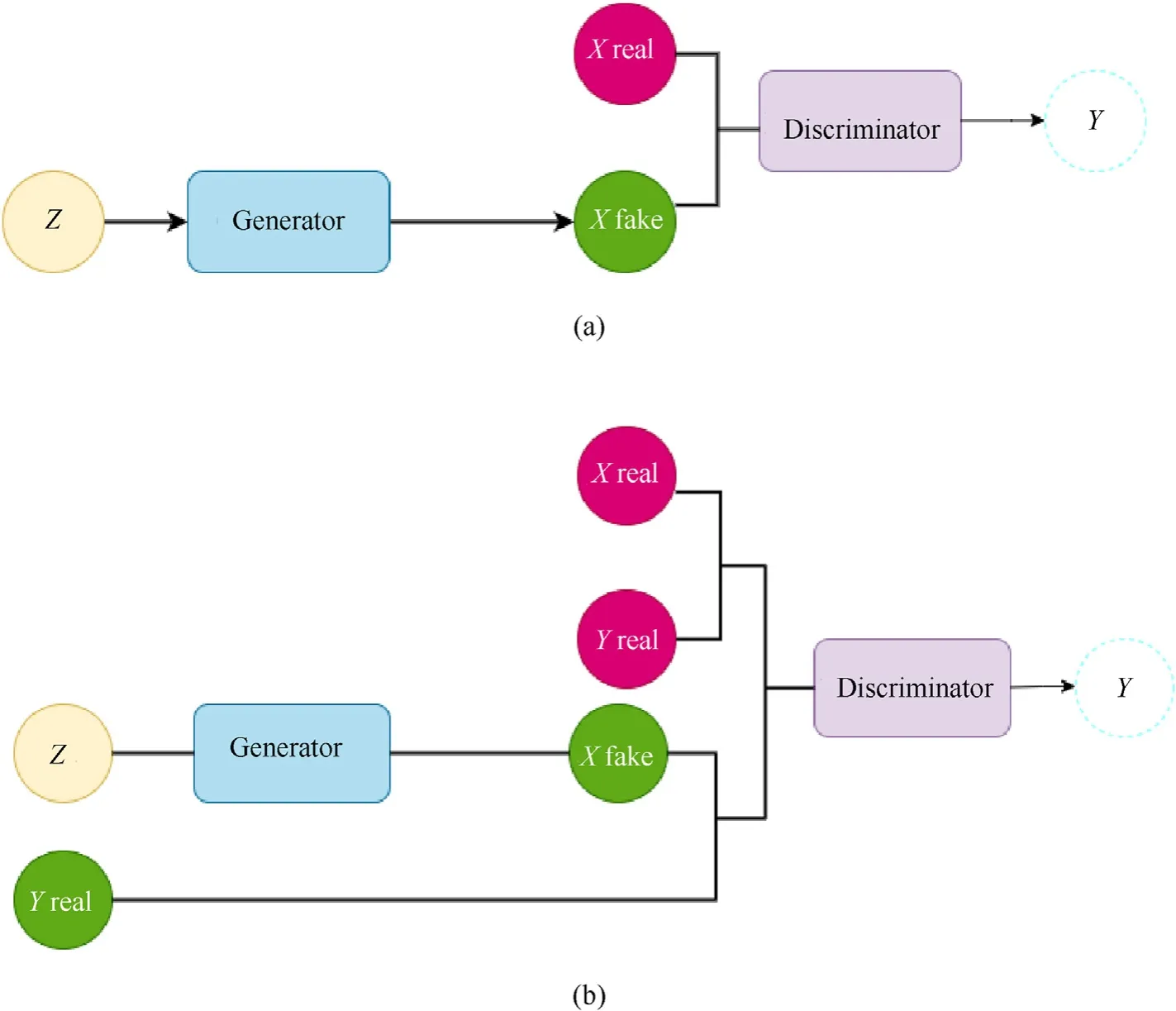
Fig. 3. Basic architecture of GAN and CGAN Models: (a) Generative Adversarial Network. The GAN architecture is comprised of both a generator and a discriminator model. The generator basically is accountable for building new output,such as images,that possibly have come from the original dataset.The generator present in the neural network creates fake data to be trained on the discriminator,it learns to generate rational data.The generated instances become negative training examples for the discriminator.The generator aims to make the discriminator classify its output as real. The discriminator takes a fixed-length random noisy input vector and generates a sample; (b) Conditional Generative Adversarial Network(cGAN).The cGAN’s are an extension of the GAN model.The conditional generative adversarial network also takes the benefit of labels while training data.The generator is given a label and random array as input that aims to solve the problem by telling the generator to generate images of a particular class only, which further helps the generator to create examples very similar to the real dataset.

The output from the algorithm is label-dependent where cGAN model has two key components-a U-Net Generator and PatachGAN Discriminator [54]. The U-Net architecture segments the objects from images that are given as input to the generator. The architecture has two paths,first path is used to capture the context in the image and is a contraction path, called the encoder. The encoder takes the grayscale image and produces a latent representation of it.On the other hand,the second path is symmetrically expanding path that enables precise localization using transposed convolutions. The decoder’s job is to produce an RGB image by enlarging this produced latent representation.The generator has an encoderdecoder structure with layers placed symmetrically.The Generator tries to increase the error rate while the discriminator tries to reach an optimal solution to identify fake images.The model is based on Game Theory and after some time, the generator and the discriminator reach a Nash equilibrium which means one component maintains its status regardless of the actions of the other component [48]. The generator and the discriminator are the neural networks that run alternatively in the training phase. The path is repeated a number of times, and the discriminator and generator both get finer with each repetition of steps in the layers. For the number of steps considered in the algorithm, in one step, the generator runs once and the discriminator runs twice. The generator takes the grayscale image and outputs an RGB image.

In paired image-to-image translation the sole purpose of the discriminator abides in examining the real and fake examples.The real sets of images are fed to discriminator from the original dataset,while the fake data comes from the generator.The purpose of the generator resides in producing images so realistic that discriminator is convinced the images are real. Over the time application of backpropagation to update biases and weights of the models, the generator steadily learns to build the samples that mimic both physical and mathematical distribution of the original dataset.The similarities between the two images(ground truth and prediction) are determined by calculating theL2 norm. For instance,L2 norm between the two imagesI{1}andI{2}is defined as

Here,subscriptsl,mrefer to one pixel in the images,andn=1,2,3 represents the three channels red, green, blue (RGB) of the image colors. Furthermore, as the images generated from the generator are able to convince the discriminator, a secured value is obtained for the correlation factor. The correlation factor between the two images is given as Ref. [48].

As mentioned before, the correlation factor becomes better with the decrease in loss function of the generator. With the increasing degree of accuracy, the model can further be useful in fast prediction of physical fields in the composites with geometric information in image-based description.

2.3. Coupled machine learning assisted algorithm for composites

Purely data-driven mapping of input and output quantities of interest through machine learning has widely been investigated in the context of composite materials and structures [56—66]. In the present study, we incorporate image-based learning [35,54] for better performance in the microstructural characterization of composite materials. The GAN framework incorporates generator and discriminator where both are neural networks. Both these neural networks with different architectures tend to produce several types of GANs[55].Here,cGAN uses CNNs as the generator and discriminator where discriminator is a classifier that classifies whether the image received is an original image or if it is generated by the generator(refer to Fig.4 and Fig.5).The input data is fed in the pix2pix GAN where it controls conversion of a given source image to the original image. The image-to-image translation requires specialized models and loss functions for a given translation of dataset. Accordingly, cGAN provides a condition on the input image for generating the target image and implements it in pix2pix GAN which further changes the loss function and uses a condition on the input image in order to obtain generated data that resembles the real data. In this work,we couple the machine learning model with finite element simulations. The main aim of this study is to capture the full field stress under varying mechanical properties of the constituents for a given microstructural configuration in the elastic regime. The data generates points using Abaqus by varying Young's modulus of the carbon fibers and the epoxy within±30%of their nominal values, which are 2.8—5.2 GPa for neat epoxy and 157.5—292.5 GPa for carbon fibers.There are 256 values generated for Young's modulus of both carbon and epoxy based on Sobol sequence in the mentioned ranges.Sobol sequences are given at the base of 2 and are an example of quasi-random low-discrepancy sequences that are used to generate well-distributed points in the sample space. Note that the sample size of 256 is finalized here based on a convergence criteria considering prediction accuracy.Primarily,the simulations are run for all the 256 pairs for values of Young's modulus using Abaqus scripting, and then odb files are stored for the set of pairs.The images are then resized and modified for best performances using python script to generate training data for the ML model (refer to Fig. 6). We have investigated different schemes for the training data generation and subsequently testing the accuracy. A detailed description of such stage-wise chronological developments is given in the following section. Among the 256 samples, we have divided them into training and testing sample sets for ensuring prediction accuracies corresponding to unseen samples,the details of which are provided in the following section.

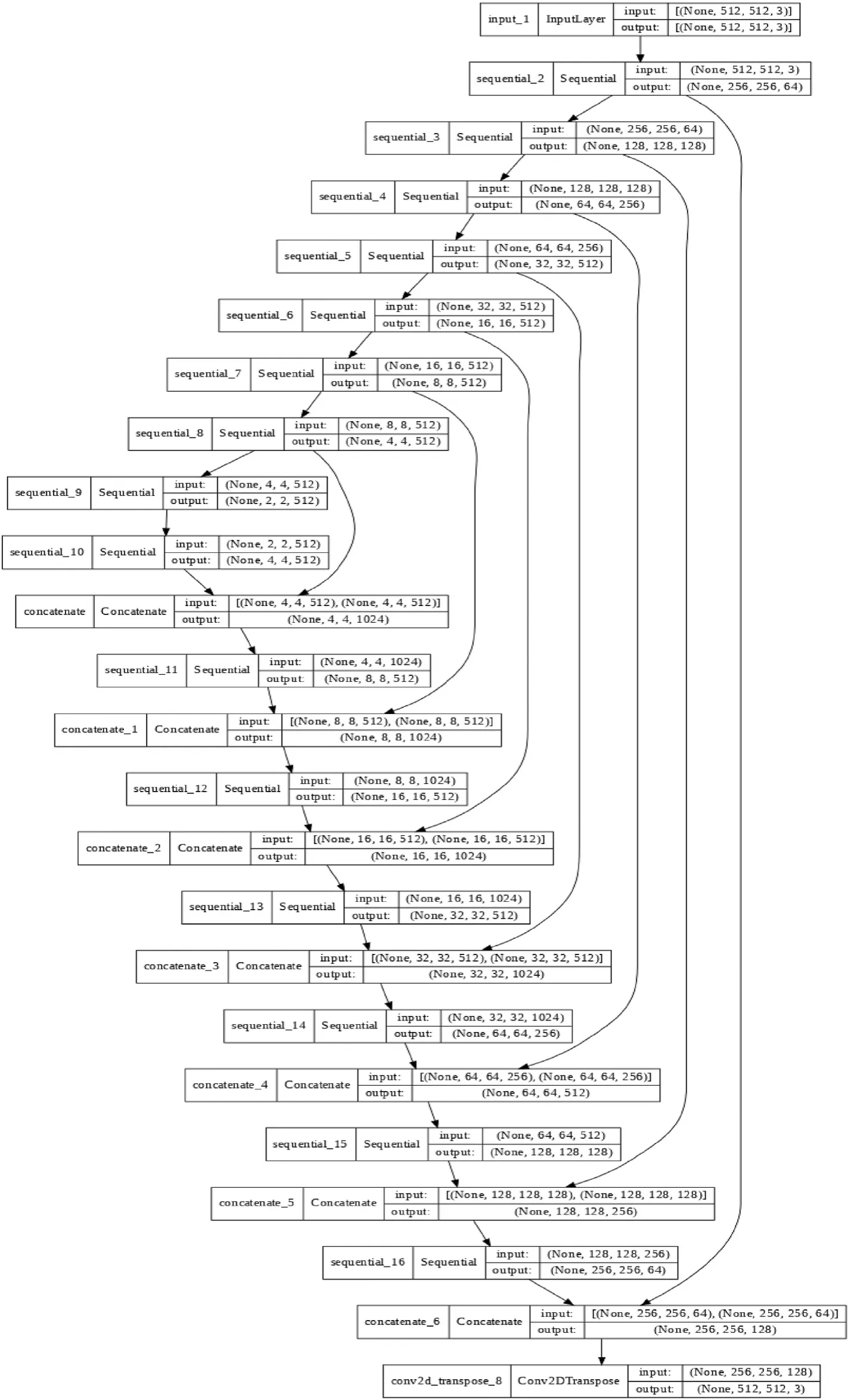
Fig.4. Layers used in the Generator.There are two types of layers in the generator model that consists of the upsampling layer that simply doubles the dimensions of the input and the transpose convolutional layer that performs an inverse convolution operation. In the GAN architecture, upsample input data is used in order to generate an output image.Upsampling layer is simple and effective, it performs well when followed by the convolutional layer. The transpose convolutional layer is an inverse convolutional layer that collectively upsamples input and learn to fill details during the model training process.

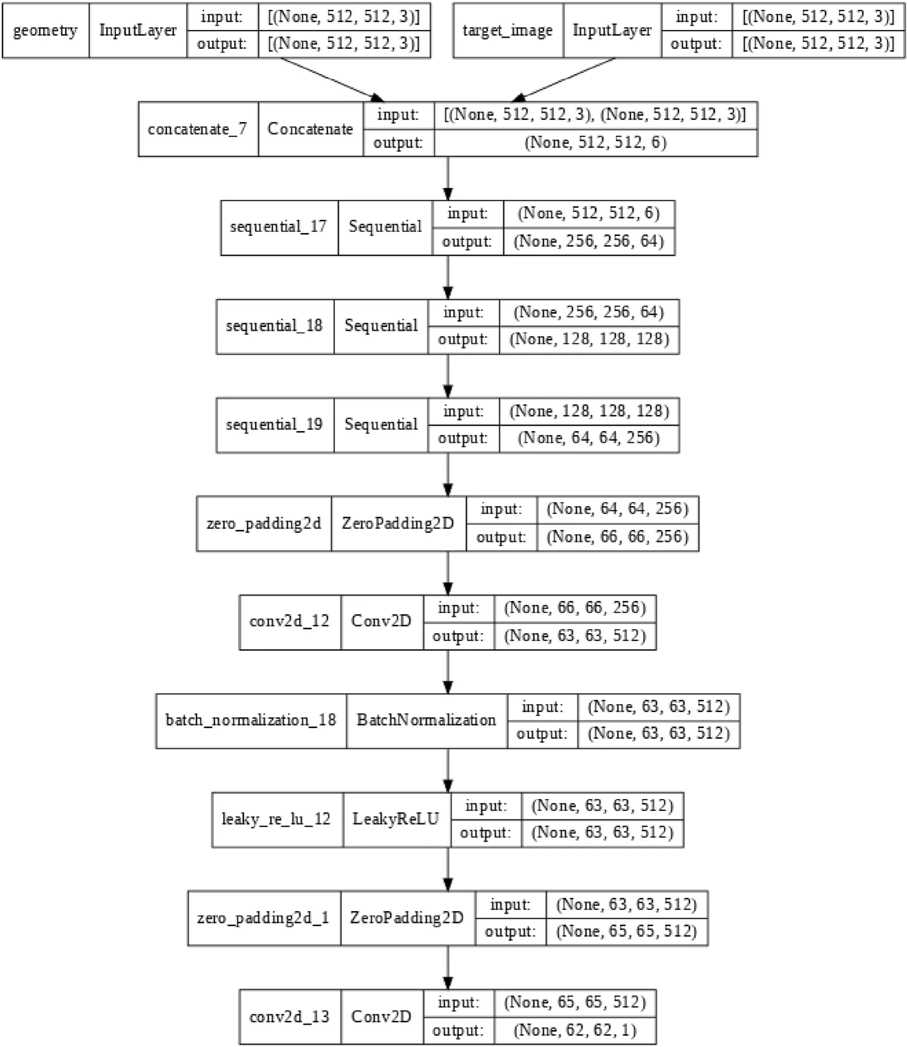
Fig.5. Layers used in the Discriminator Model.The discriminator in a GAN is termed as a classifier as it classifies both real data and fake data from the generator.The training data for the discriminator comes from two sources-real data(original set of data)and fake data(created by the generator).It distinguishes real data from data created by the generator.The discriminator uses the real data as positive examples during training whereas fake data is used as negative examples during the training.

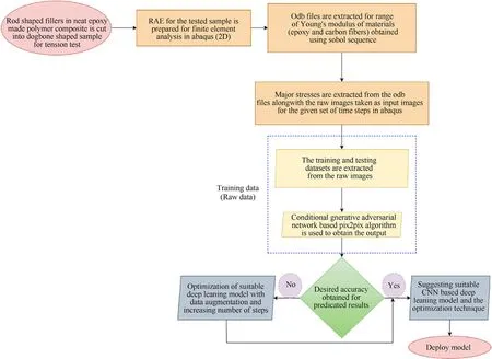
Fig. 6. Deep learning-assisted optimization algorithm. The flowchart represents the steps followed for obtaining a suitable CNN-based deep learning model from the extracted training and testing datasets of a 2D RAE of the tested sample from FEA code. The deep learning assisted cGAN is used for obtaining the accurate output from paired pix2pix translation model which particularly is a more powerful and accurate way of solving classification problems.

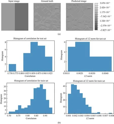
Fig.7. Typical representation of the pix2pix input images with contours turned off in ground truth and received predicted results along with the correlation factors and L2 Norm for train and test sets(Model 1).(a)Representative black to white spectrum output images.The input image in the pix2pix model is in the form of an image of 512×512 dimensions.The input image comprises two parts,where the left part represents Young's modulus of the epoxy and the right part represents Young's modulus of carbon.The model consists of the ground truth and predicted images along with the obtained correlation factor and L2 norm;(b)The results of correlation and L2 norm are obtained for the given sets of train and test data.

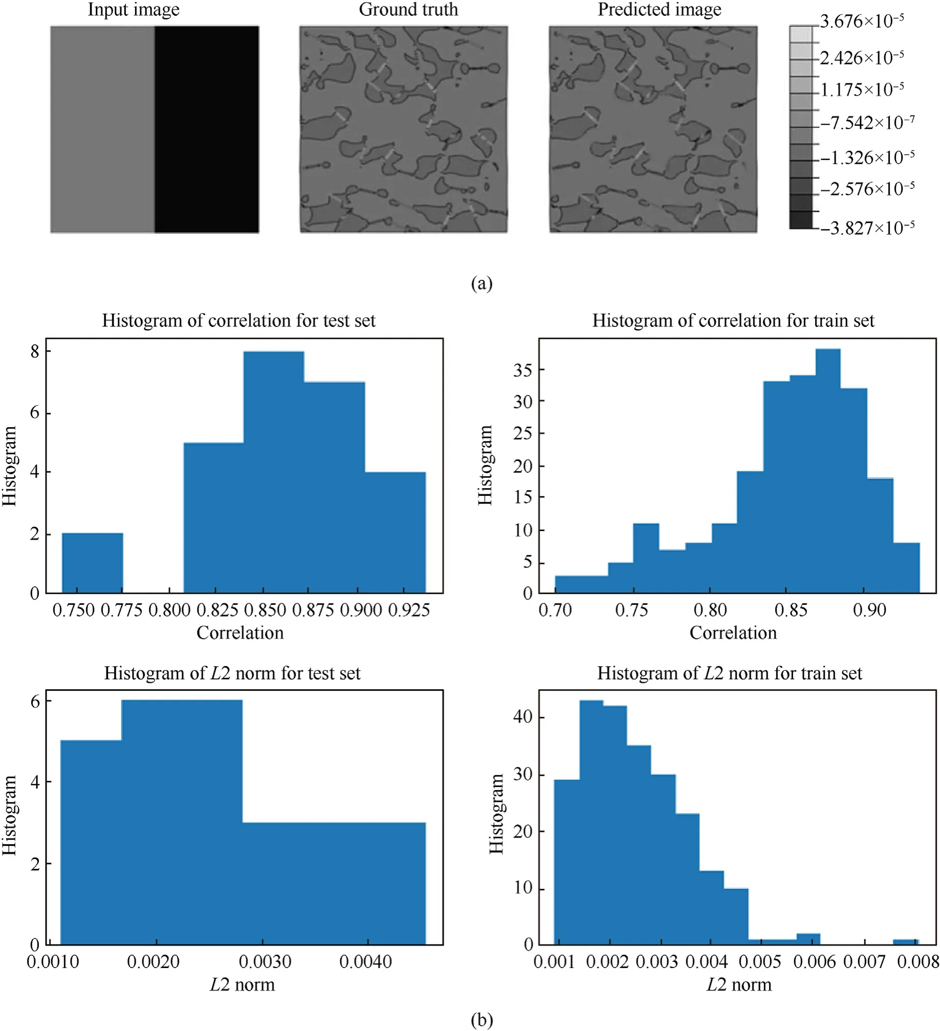
Fig.8. Typical representation of the pix2pix input images with contours turned on along with ground truth and predicted results including the correlation factors and L2 Norm for train and test sets(Model 2).(a)Representative black to white spectrum with contours turned on.The contours are turned on in composite for more apparent variation of stresses in the output.It becomes feasible for the model to observe and learn the variations in the images as the shape of contours in the images are also changing along with the changes in the colors; (b) The results of correlation and L2 norm are obtained for the given sets of train and test data.

Fig.9. Typical representation of the pix2pix input images with the rainbow spectrum including ground truth and predicted results along with the correlation factors and L2 Norm for train and test sets (Model 3). (a) Rainbow spectrum in Abaqus is obtained for the model, which means that the stress from the single pixel is represented with the help of 3 dimensions. The colors are represented using RGB colour values; (b) The results of correlation and L2 norm are obtained for the given sets of train and test data.

3. Results and discussion

The training process is a very crucial step in the implementation of cGAN, wherein the generator and discriminator are optimized such that the loss functions of both the generator and discriminator are satisfied for creating minimum error and desired correlation of value closer to 1.It is observed that for achieving a good correlation in the ground truth and predicted results, the loss function of discriminator has to perform two tasks, firstly, it has to accurately label real images as ‘real’ coming from the training data and secondly, it must correctly label images as ‘fake’ for the generated data coming from the generator. In this study, the RGB images are converted to grayscale which acts as the input data for our model.The pix2pix model requires input in the form of an image and the size of the input image is chosen 512×512 dimensions.This section consists of training data generation through a number of models(Model 1 to Model 8) and we have further verified the accuracy of predicted results in the form of correlation and L2 norm of the specified inputs.The output received for the predicted images is in the form of RGB image. The whole work has revolved around the tensor flow library that requires a Graphical Processing Unit(GPU)for its ability to efficient, smooth, and optimized execution on the computer system.

Model 1 is created for black to white spectrum output images,where the image input is divided into two parts.The left part of the input image represents Young's modulus of the epoxy and the right part represents Young's modulus of the carbon. The values of stresses are linearly scaled between 0 and 255 representing the colour in greyscale. The first 256 samples of the Sobol sequence generated for two variables are divided into a training set consisting of 230 images and a testing set consisting of 26 images.However, it is observed that the model is not able to capture the variations in the stresses and is stuck in the local minimum. The variations in the predicted image are very small which means that the model has found an image that is optimum to predict for all the cases (refer to Fig. 7).

In Model 2,similar images are passed as for the case in Model 1 with the only difference that the contours are turned on for showing the variation of stresses more apparently in the output.This could make it easier for the model to observe and learn the variations in the image. Consequently, along with the changes made in contours, the shape of contours in the images is also changing.However,the observations in the predictions remain the same like in the case of contours turned off. The model is found stuck in the local minimum.Also,it predicts very similar images for all the input images (refer to Fig. 8).

Model 3 has shifted from black to white spectrum and used the rainbow spectrum in Abaqus. Each of the three parameters (red,green, and blue) defines the intensity of the colour as an integer between 0 and 255. Additionally, the higher dimension can represent the colors with higher accuracy.The observations made for the model captured certain variations in the stress field but not with perfect accuracy. Despite that, some samples have shown good results and the problem of predicting very similar images for all the samples is avoided.Model 3 is found to give more improved results over the last two models (refer to Fig. 9).

Model 4 follows the previous case with the only difference of contours enabled just as in model 2. The model is designed such that it is able to capture changes in images better since there are shape changes in addition to colour changes. However, the model has performed accurately in regions where there is a lot of variation in contours.The changes in the stresses are captured accurately by the model for some cases and there are improvements seen in this case as well over the previous three models (refer to Fig.10).

Fig.10. Typical representation of the pix2pix input images with the rainbow spectrum including ground truth and predicted results along with the correlation factors and L2 Norm for train and test sets(Model 4).(a)Representative plots in rainbow spectrum with contours enabled.The current model is the same as Model 3 with the only difference being that the contours are enabled. The model is such that it captures changes in images for additional shape changes along with the colour changes; (b) The results of correlation and L2 norm are obtained for the given sets of train and test data.

Model 5 incorporates time steps along with the earlier used parameters which include varying Young's modulus of carbon and epoxy in the composite.The stresses are varying in the material as the time steps are varying in Abaqus. Time is captured by variable frame number in Abaqus which is referred to as time step,wherein the simulation includes time step from 0 to 102.All-time steps are included in the training data and the input image is given with a different colour strip for time steps.There are 6-time steps taken in the range from 15 to 90 and are linearly scaled to the range 0—255,which act as the greyscale value,representing frames.The model is prepared for 1350 training and 415 testing images using Young's moduli created with Sobol sequences. In this context, it can be noted that we are increasing the training samples here significantly,while the number of finite element simulations still remains the same. This is because of the fact that no additional finite element simulations are required for capturing the images corresponding to different time steps. It is found that this model predicts the contours accurately for almost all samples barring from a few initial time steps with very low stresses. However, these contours also create noise in the model.The predictions obtained suggest giving the ground truth images to the pix2pix model with contours turned off could obtain better results (refer to Fig.11). We also note here that it becomes difficult to distinguish between different stresses in the full field images since the range of stress is very high.We try to address these issues in the subsequent models.

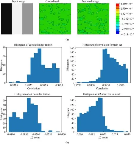
Fig.11. Typical representation of the pix2pix input images with additional time-step parameter including ground truth and predicted results along with the correlation factors and L2 Norm for train and test sets(Model 5).(a)The additional parameter in the input image includes time.The model is prepared such that it has an additional parameter of varying time steps along with the changing Young's modulus for carbon and epoxy in the composite.Time steps are captured by the frame number in Abaqus which is referred to as time steps. The Timestep is represented in the input image in the same way Young's modulus variations are represented. The model consists of three columns in the input images,representing, Young's modulus of epoxy,Young's modulus of carbon,and time step respectively.The contours in the model make it easier to distinguish between different images but also introduce some noise to the model. (b) The results of correlation and L2 norm are obtained for the given sets of train and test data.

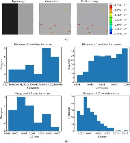
Fig.12. Typical representation of the pix2pix input images with either in black or grey based on whether the values are higher or lower than the current spectrum,including ground truth and predicted results along with the correlation factors and L2 Norm for train and test sets(Model 6).(a)It represents training for S11min to-1.03×10-5 spectrum,where S11 is the minimum stress observed in the composite.The image generated for the sample representing the spectrum consists of part of the composite not present in the spectrum.This makes the stresses in the epoxy region become apparent and can be easily learnt by the model.(b)The figures represent the results of the correlation and L2 norm for input images corresponding to S11min to -1.03 × 10-5.

Fig.13. Typical representation of the pix2pix input images with either in black or grey based on whether the values of training lie in -1.03 × 10-5 and 8.83 × 10-4 spectrum,including ground truth and predicted results along with the correlation factors and L2 Norm for train and test sets (Model 6). (a) The model corresponds to a different range of stresses.It represents the same features as Model 6 in Fig.10 and concerns training for-1.03×10-5 and 8.83×10-4 spectrum;(b)Representation of the Histogram of train and test set showing L2 norm and correlation factor.

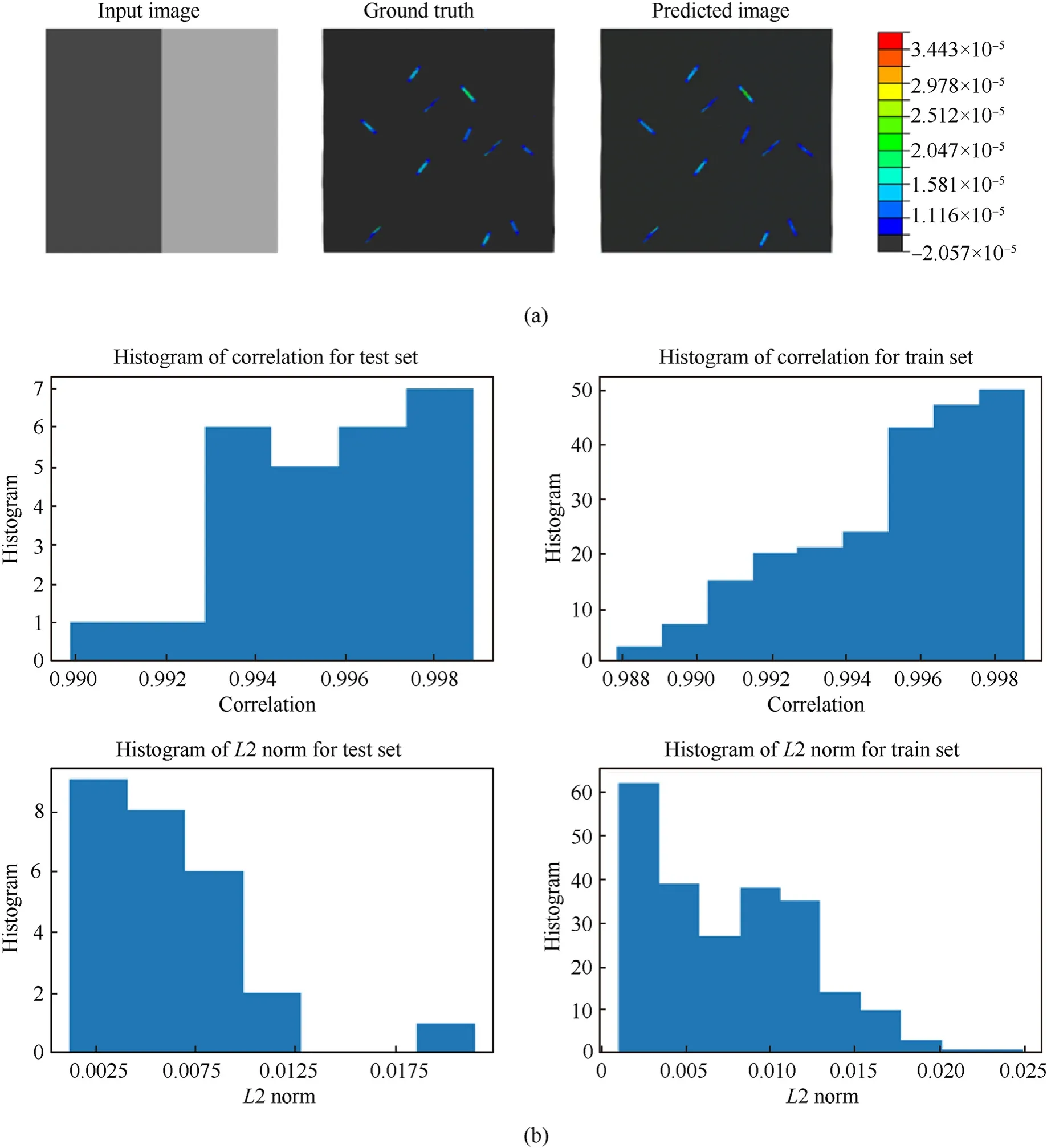
Fig.14. Representation of Model 6 training for 8.83×10-4 to S11max spectrum where S11max is the maximum stress in the composite.(a)Stress contour in the specified range.The black corresponds to the value of stress in the material below the minimum stresses.It means the black part does not lie in the chosen spectrum and is not the area of interest.(b)The graphs represent the correlation and L2 norm of the considered train and test dataset.

Model 6 is created to train for three different spectrums of stresses to address the issue of high stress variation in the entire domain.The other modeling attributes are kept the same as that of Model 4 here. The uniform green color in the epoxy shows a low magnitude of stress as compared to the carbon fibers in Fig. 10.Keeping that in view,the stresses are split into three equally spaced ranges and the mean of the values form the boundary of these ranges.These averages come out to be:1.03×10-5and 8.83×10-4.So, all the results are split into three ranges:S11minto -1.03 × 10-5, -1.03 × 10-5to 8.83 × 10-4,and 8.83 × 10-4toS11max, whereS11minis the minimum stress observed in composite andS11maxis the maximum stress in the composite.Three different images are generated for each sample representing different spectrums and the part of the composite that is excluded from the stress range spectrum has painted either black or grey based on if the values are higher or lower than the current spectrum.Following this model makes the stresses in the epoxy region more apparent and the stress field can be learned by the model more precisely.The model is trained without considering the time steps. Figs. 11—13 show that Model 6 can predict the variation in stresses very well for the spectrum-10-5to 10-5,while the model gave conservative results for the other two ranges.This model predicts similar images for all samples as in the case of observation made in Model 1 and 2.Another obstacle in using this approach is that some fibers lie in one spectrum for some values of Young's modulus while in another spectrum for some other values of Young's modulus. This has led the model to predict carbon fiber in some instances even when it is absent in the ground truth. Despite this, the model has also given promising results, which motivated us to improve this model further (refer to Figs.12—14).

Model 7 takes a different approach to deal with the stress range,wherein the input images are divided into two images for each sample. The two output images for carbon and epoxy exhibit different colour bars; hence representing different ranges of stresses. Different models are trained for both the image sets. It is found that the model predicts the stresses quite accurately for both carbon and epoxy(refer to Fig.15 and Fig.16).However,the results can be further improved if we split the output images into different spectrums of stresses, specifically for the positive and negative stress ranges considering the fiber and matrix separately.

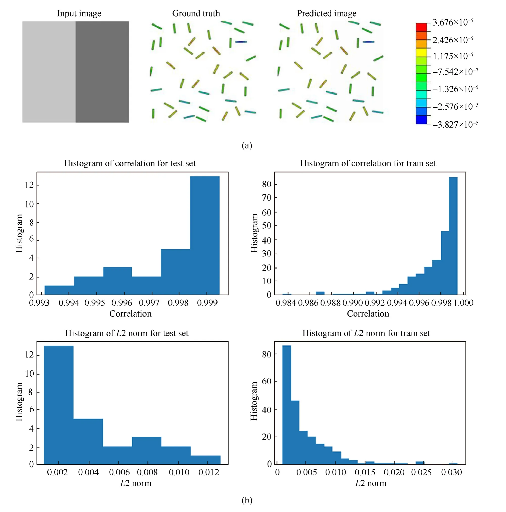
Fig.15. Representation of stress field prediction only in fibers(Model 7).(a)The model shows the results for stresses developed in the carbon fibers.The model accurately predicts stresses in the carbon fibers for the given range of stresses.(b)The graphical representation gives an interpretation of the results of the L2 norm and correlation factor between the ground truth and predicted images.

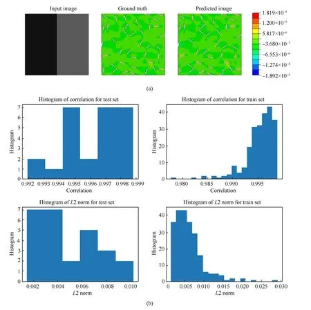
Fig. 16. Representation of stresses developed in epoxy matrix for Model 7. (a) The model predicts the results for the stresses developed in epoxy, wherein a good prediction capability can be noticed. (b) The graphical representation of the output in the form of L2 norm and correlation factor.

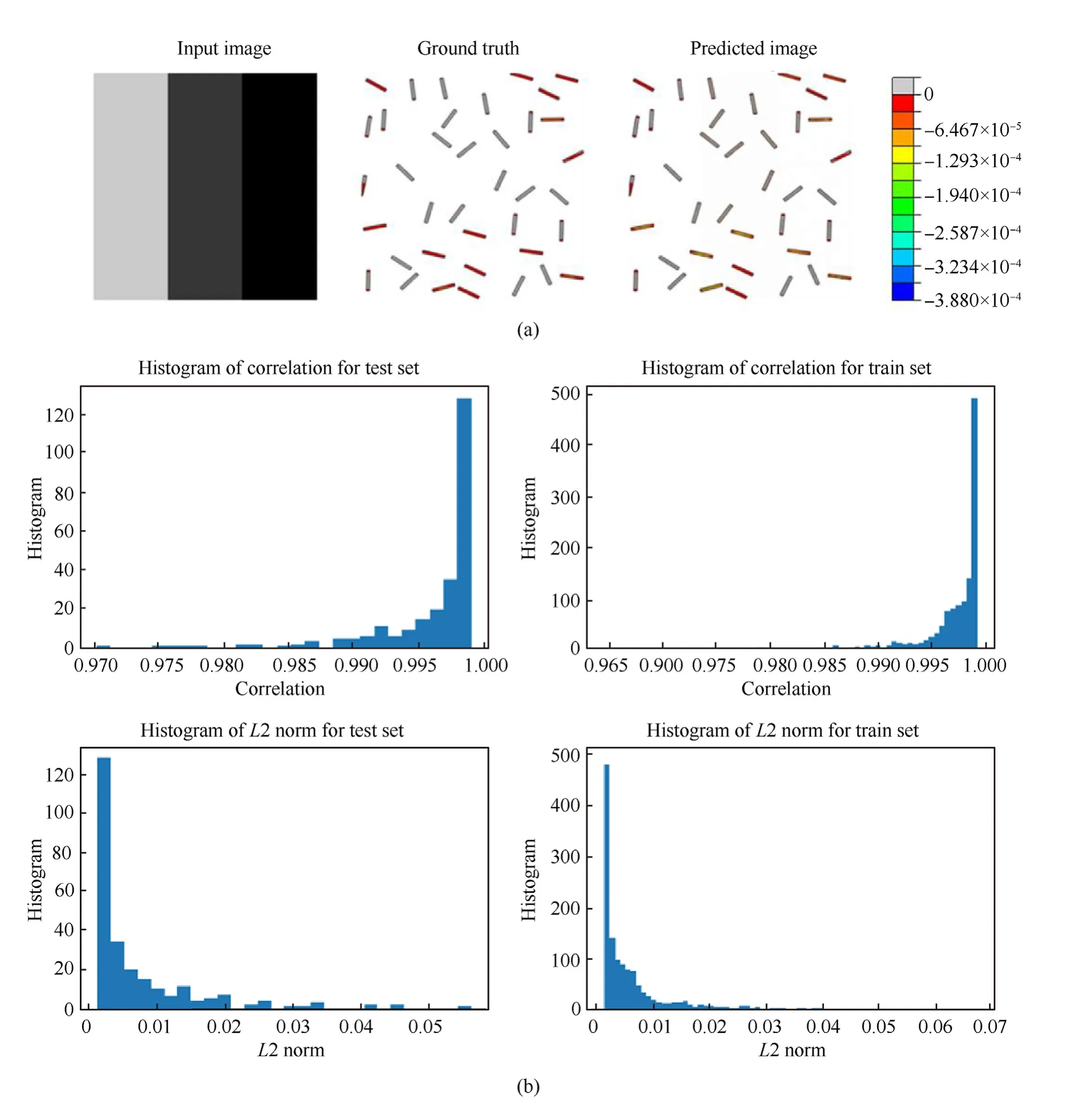
Fig.17. Typical representation of the negative stress spectrum in carbon fibers(Model 8).(a)This model predicts results for the negative spectrum of carbon fibers.The models in this case are separated for the negative and positive range of stresses for both the materials. There are four different models created under Model 8 for the lower limit and upper limit of stresses for each case of the material. (b) The results are found to be in good agreement with negative stresses developed in the carbon fibers and the plots show high correlation factor with low value of the L2 norm.

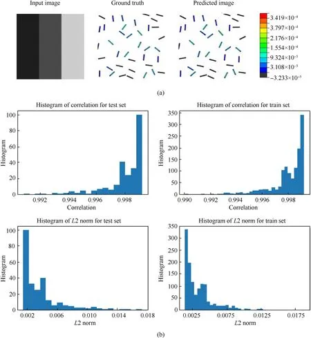
Fig.18. Typical representation of the positive stress spectrum in carbon fibers (Model 8). (a) This model predicts results for the positive spectrum of carbon fibers. The models in this case are separated for the negative and positive range of stresses for both the materials. There are four different models created under Model 8 for the lower limit and upper limit of stresses for each case of the material. (b) The results are found to be in good agreement with positive stresses developed in the carbon fibers and the plots show high correlation factor with low value of the L2 norm.

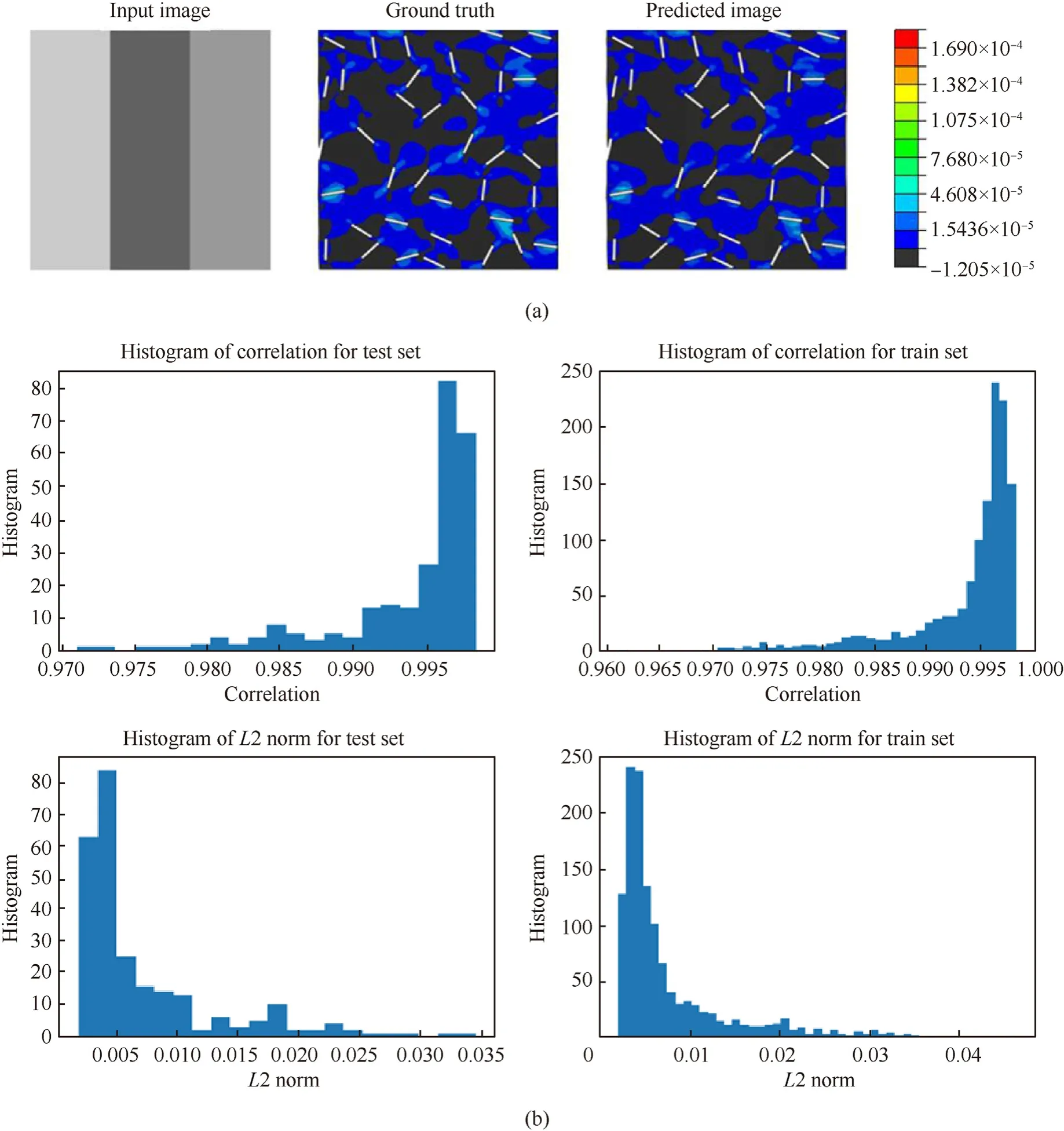
Fig.20. Typical representation of the positive stress spectrum in epoxy(Model 8).(a)This model predicts results for the positive spectrum of epoxy matrix.The models in this case are separated for the negative and positive range of stresses for both the materials. There are four different models created under Model 8 for the lower limit and upper limit of stresses for each case of the material.(b) The results are found to be in good agreement with positive stresses developed in the epoxy matrix and the plots show high correlation factor with low value of the L2 norm.

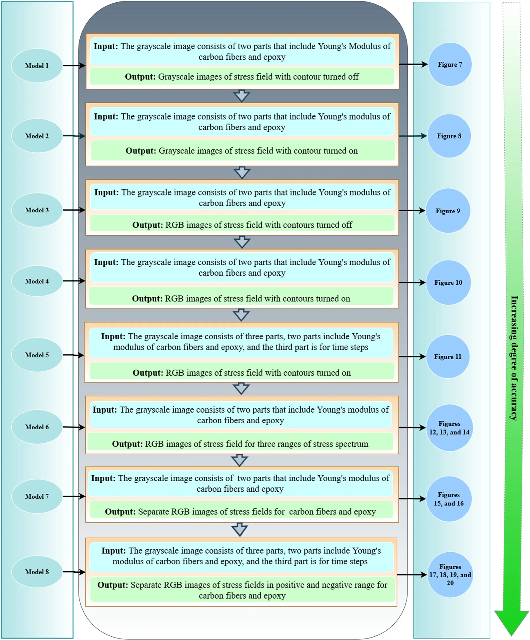
Fig.21. Chronological development and descriptions of the models.The figure shows the specific descriptions of the input and output images(Model 1 to Model 8)for training and testing sets along with the respective figures representing the results (refer to Figs. 7—20).

Model 8 improves the Model 7 by incorporating different output images based on positive and negative stress ranges.In addition to training the different models for carbon and epoxy as in Model 7,the positive and negative ranges of the spectrum representing stresses are separated in Model 8.In this case,a total of four models are trained for each carbon and epoxy corresponding to the positive and negative spectrum of stresses as shown in Table 2.Model 8,in addition to the upper and lower limit of stresses, incorporates the time steps variable as followed in Model 5. This is done based on the clear understanding that incorporation of time step to increase the training data improves the accuracy(as shown in Model 5).The Model 8 consists of six-time steps at regular intervals of 15,30,45,60, 75, and 90. The model can affirmatively predict the stresses with a reasonable degree of accuracy, wherein it is observed to obtain outputs very close to the ground truth(refer to Figs.17—20).

Table 2Limits of stress in colour spectrum corresponding to neat epoxy and carbon fibers.

A concise description of all the models according to their order of development and level of accuracy is provided in Fig. 21. The purpose of the model validation here is to make the ML model accurate enough for having adequate reliability. It concerns the identification and elimination of errors in the learning of data. An L2 Norm of less than 0.005 for most of the samples in the spectrums is achieved in Model 8,which refers to the accuracy obtained in the generated images from the generator.Thus the cGAN-based Model 8 predicts the principal stress in thex-direction (S11) with an acceptable degree of accuracy. The cGAN-based model has satisfactorily learned to predict the stress distribution for the given geometry, the position of fibers, loading, and boundary conditions through generator and discriminator. The discriminator is trained in such a manner that it has given output probabilities closer to 1 for real images (from the dataset). Thereupon the generator is trained to forge such realistic images that it makes the discriminator output probability closer to 1 even for forged images(images from the generator). The effective learning of the cGAN-based DL model is justified by the obtained results for stress distribution closer to ground truth images in the case of both carbon fibers and neat epoxy. It is observed that the problems encountered in the other models, where the generated data is unable to trick the discriminator and inefficient to create results as good as Model 8,have been sorted in the final model. As a result, the stress distribution in the predicted results is found to be very similar to ground truth in comparison with the other input methods opted in the previous models.

4. Conclusions

This paper proposes a deep learning model such that it takes the microstructural image as input with a different range of Young's modulus of carbon fibers and neat epoxy, and obtains output as visualization of the stress componentS11.For obtaining the training data of the ML model, a short carbon fiber-filled specimen under quasi-static tension is modeled based on 2D Representative Area Element(RAE)using finite element analysis.The study reveals that the pix2pix deep learning Convolutional Neural Network (CNN)model is robust enough to predict the stresses in the composite for a given arrangement of short fibers filled in epoxy over the specified range of Young's modulus with high accuracy.The CNN model achieves a correlation score of about 0.999 andL2 norm of less than 0.005 with adequate accuracy in the design spectrum, indicating excellent prediction capability. In this paper, we have focused on the stage-wise chronological development of the CNN model with optimized performance for predicting the full-field stress maps of the fiber-reinforced composite specimens. Among different prospective models, which are explored in this study, Model 8 shows the best prediction accuracy. In this model, we have divided the stress field for fiber and matrix into their respective positive and negative stress spectrums. We further show that along with the respective Young's modulus of matrix and fibre, the inclusion of time step as input level improves the prediction accuracy significantly without any additional cost of finite element simulation.

In summary, the cGAN is capable of satisfactorily learning to predict the full-field stress distribution in composites for the given geometry, boundary conditions, and loading condition. The development of such a robust and efficient algorithm would significantly reduce the amount of time and cost required to study and design new composite materials through the elimination of numerical inputs by direct microstructural images. The proposed approach may be extended to explore other stress and strain components along with various failure criteria. The new developments in the paper would contribute significantly toward direct image-based data-driven predictions, which will accelerate the microstructural analysis of composites and bring about novel efficient approaches for innovating and designing multifunctional materials.

Declaration of competing interest

The authors declare that they have no known competing financial interests or personal relationships that could have appeared to influence the work reported in this paper.

Acknowledgments

SG and VK would like to acknowledge the financial support received from DST-SERBSRG/2020/000997,India.TM acknowledges the initiation grant received from IIT Kanpur. The authors are thankful to Achint Agrawal(IIT Kanpur) for his contribution to the initial developments of the CNN algorithm for this work.