Streamflow prediction in ungauged catchments by using the Grunsky method
Bruno K.Mrchezepe , Andrˊe Almgro , Andrˊe S.Bllrin , Pulo Trso S.Oliveir ,,*
a Department of Hydraulics and Sanitary Engineering, São Carlos School of Engineering, University of São Paulo, São Carlos, SP, Brazil
b Faculty of Engineering, Architecture and Urbanism and Geography, Federal University of Mato Grosso do Sul, MS, 79070-900, Brazil
Keywords:Regionalization Hydrological group Temporal scale Tropical basins
A B S T R A C T Establish a reliable rainfall-runoff relation capable of predicting runoff in ungauged basins is a matter of interest across the world for a long time and has been taking importance during the past decades.Regionalization approaches, hydrological models and machine learning techniques have been used to estimate runoff.However, returning some simplicity to the predictions might be necessary for practical uses.In this paper, we re-introduce C.E.Grunsky approach, developed in the early 1900s to predict runoff from values of precipitation on a two-equations system.Here,we analyze the Grunsky generalized method applied for 716 Brazilian catchments,on an interannual and monthly scales.First,we established the best method to find the rainfall-runoff relation coefficient for each catchment.Then,we evaluate the performance of the method on a local scale,i.e.,catchment by catchment.Lastly,we analyze the method of regionalization, by grouping the catchments into six hydrologically similar classes.For local scale, the Kling-Gupta Efficiency (KGE)values range from 0.87 to 0.93 on the interannual scale and is greater than 0.50 on the monthly scale.For the regionalized approach,KGE varies from 0.60 to 0.84 on an interannual scale.We also found suitable KGE values on a monthly scale,with more than 22%of catchments with KGE greater than 0.50, being the best performances in the Non-seasonal and Extremely-wet groups, and the worst performance in the Dry group.Our findings indicate that Grunsky approach is suitable to predict streamflow for Brazilian catchments on interannual and monthly scales.This simple and easy-to-use equation presents a reliable alternative to more complex methods to compute runoff by only using rainfall data.
1.Introduction
The understanding of the nature of temporal and spatial variability of hydrological fluxes, especially runoff, is crucial for hydrological studies, design of hydraulic structures, and water resources management (Beck et al., 2015; Dal Molin et al., 2020;Viglione et al., 2013).Despite its importance, the correct understanding of catchments’hydrological behavior remains a challenge,given that most basins across the world are ungauged, which precludes a precise temporal and spatial characterization.Due to this lack of data,the study of the prediction parameters in those basins has received a great deal of attention in the last decades (Razavi et al., 2012; Bloschl & et al., 2013; Salinas et al., 2013).
Several methods have been widely used for streamflow prediction,such as the Rational Method proposed by Thomas Mulvany(Dooge, 1974), the Synthetic Unit Hydrograph (Snyder, 1938), the Soil Conservation Service - SCS Curve Number (United States Department of Agriculture, 1986, p.164), and physically based(e.g.TOPMODEL,Beven,1997)and conceptual hydrological models(e.g.HBV,Seibert&Bergstr¨om,2021).Throughout the years,these methods received contributions, and improvements, and were tested in many studies around the world (Bhunya et al., 2011; Fan et al., 2013; Grimaldi & Petroselli, 2014).Nevertheless, some of these methods have inherent limitations and drawbacks, such as the(i)subjectivity present in parameter selection and their lack of interpretability and the (ii) low reproducibility of the models in different spatial and temporal scales (Young et al., 2009; Bhunya et al.,2011;Fan et al.,2013;Hrachowitz et al.,2013)that results in increased uncertainties and a challenging scenario for model selection (Grimaldi et al., 2013; Grimaldi & Petroselli, 2014).
Most recently, an initiative of the International Association of Hydrological Sciences called the Decade of Predictions of Ungauged Basins (PUB) 2003-2012 (Sivapalan et al., 2003) and 2013-2022(Montanari et al., 2013), sought to merge the knowledge gathered so far,in an attempt to better summarize the core questions and the benefits and drawbacks of each model (Hrachowitz et al., 2013).Nevertheless, both PUB initiatives struggled in unifying and summarize the modeling strategies.Thus, different approaches have been proposed and applied since then,with no scientific consensus(Bloschl & et al.,2013; Yang et al., 2020; Pool et al., 2021).
Since the released of the PUB initiative,and particularly within the last decade, numerous changes have taken place in hydrolical modeling approaches.From worldwide high-resolution data availability (Abatzoglou et al., 2018; Brown et al., 2022; Velthoven et al., 2021) to the development of sophisticated methods that incorporate machine learning approaches,such as Artificial Neural Networks (ANN), Random forest, and Long Short Term Memory(LSTM) methods.Despite exhibiting a good performance even for sub-daily predictions and for data-scarce areas (Ayalew et al.,2022), machine learning approaches need large datasets to be trained, do not often offer transparency in terms of process understanding, and require further investigation to quantify uncertainties associated to predictions (Kasiviswanathan & Sudheer,2017; Seo et al., 2018).In addition, in terms of prediction quality,they do not differ from stochastic methods,which enforces the idea that there is no perfect prediction method for all circumstances(Mehdizadeh et al., 2019; Papacharalampous et al., 2019).
In general,good performance on predictions can be reached by using the mentioned approaches,with a major challenge remaining in the choice of the best method for each circumstance,and finding gauged catchments that are good parameters “donors” for regionalization purposes(Pool et al.,2021).Moreover,despite small-scale heterogeneity and process complexity,the hydrological response at the catchment scale is often characterized by process simplicity(Beven, 2000; McDonnell, 2003; Sivapalan et al., 2003).Nevertheless, the extensively employed, traditional, and processoriented approaches could prove highly beneficial when employed in conjunction with contemporary, data-driven methodologies, enabling a more complete comprehension of hydrological processes implicated in the predictions of ungauged basins.
At the end of the 19th and beginning of the 20th century, in a scenario of the early forming of hydrology as a science and lack of computational performance,a great variety of empirical equations had arisen,searching for a reliable rainfall-runoff relation(Eview&Linsley,1967; Hubbart, 2011).One of these studies was led by the former president of the American Society of Civil Engineers(ASCE),Carl E.Grunsky(1908,1915),who developed somewhat of a“ruleof-thumb” (Santos & Hawkins, 2011), directly relating the average annual runoff(Q)to the average annual precipitation(P)in the São Francisco peninsula, located in California, USA.The author established this practical relation from hydrological observations during the 1900s decade.Despite of the simplicity of Grunsky's proposed framework,it achieved an excellent performance in describing the long-term hydrological fulxes.
More than a century after Grunsky's study with restricted information at his disposal, Santos and Hawkins (2011) generalized the method, inserting a single coefficient, called α, for studying Mediterranean catchments in California (USA), Southern France,and Portugal,with areas ranging from 1.47 to 97,667.00 km2.They reported that the proposed approach reached a coefficient of determination of 0.89 for observed and predicted annual runoff in Portuguese watersheds, and almost 1:1 relation for the French watersheds, which shows an exceptional perspective for the method, given its simplicity.Furthermore, they have shown that the α coefficient led to the possibility of application in catchments with different responses to precipitation.However, despite the possibilities, this approach has only embraced long-term data, i.e.the mean values of precipitation and runoff.In addition, the application of this approach was limited to the Mediterranean climate and has not yet been investigated using large-sample catchment datasets.Moreover, to the best of our knowledge, no study evaluated the performance of the Grunsky method to characterize streamflow fluxes at finer temporal scales.
In this study, we investigate the performance of the Grunsky framework in computing monthly and interannual streamflow in tropical catchments.To this end, we applied for the first time the generalized Grunsky method for 716 Brazilian catchments available in the Catchments Attributes for Brazil (CABra) dataset (Almagro et al., 2020, pp.1-40).Then, we proposed a streamflow regionalization based on the median α computed for each of the six Brazilian hydrological groups.Our investigation seeks to unterstand the suitability of the approach for different climate conditions.With this study, we seek to answer the following questions: Why and when to use the Grunsky method? What are the benefits and limitations of this approach? Up to what temporal scales the method can be used?Is the Grunsky framework a suitable approach to characterize and predict hydrological fluxes at finer temporal scales than long-term scales?Can this approach be regionalized to predict streamflow in Brazilian basins?We organized this study as follows: in section 2, we describe the dataset used in the study.Section 3 shows the methods used in the study as well as the approach to employing the Grunsky method on an interannual and monthly scale.In section 4, we present and discuss the results,respectively and,in section 5,we highlight the main conclusions of the paper.
2.Material and methods
2.1.Dataset
The study comprehended the use of the Catchments Attributes for Brazil (CABra) dataset (Almagro et al., 2020, pp.1-40), which contains data from 735 catchments spread over the Brazilian territory.The attributes are grouped into 8 classes, namely: topography, climate, streamflow, groundwater, soil, geology, land-use and land-cover, and hydrologic disturbance.In addition, for each catchment, there is a 30-year daily series of precipitation, streamflow, and actual and potential evapotranspiration, from 1980 to 2010,all of them containing less than 10%of missing data.From the 735 catchments,we excluded 18 catchments that presented at least one year with Observed Annual Runoff(Qobs)higher than Observed Annual Precipitation (Pobs), and one catchment that exhibited inconsistency between long-term precipitation and evapotranspiration data,remaining 716 catchments for the analysis.A list of the 19 excluded catchments is presented in the Supplementary Material (Table S1).
We used daily time series of precipitation (P) and streamflow(Q) for the climatological period between October 1st, 1980, to September 30th, 2010 as the main attributes for our analysis,comprehending 30 hydrological years.P is derived from an ensemble mean between a high-resolution ground-based reference dataset (Xavier et al., 2016) and the ERA5 reanalysis dataset(Hersbach et al., 2020) while Q is based on streamflow gauge observations over the Brazilian catchments.Daily values were resampled to annual and monthly series.Therefore, for each catchment, 30 (360) values of annual (monthly) runoff and precipitation were computed.We excluded from our analysis years(months)with at least one day with missing value to maintain the annual and monthly values comparable within the same catchment.In other words, we only consider years (months) with complete daily records.
2.2.Re-introducing the Grunsky method
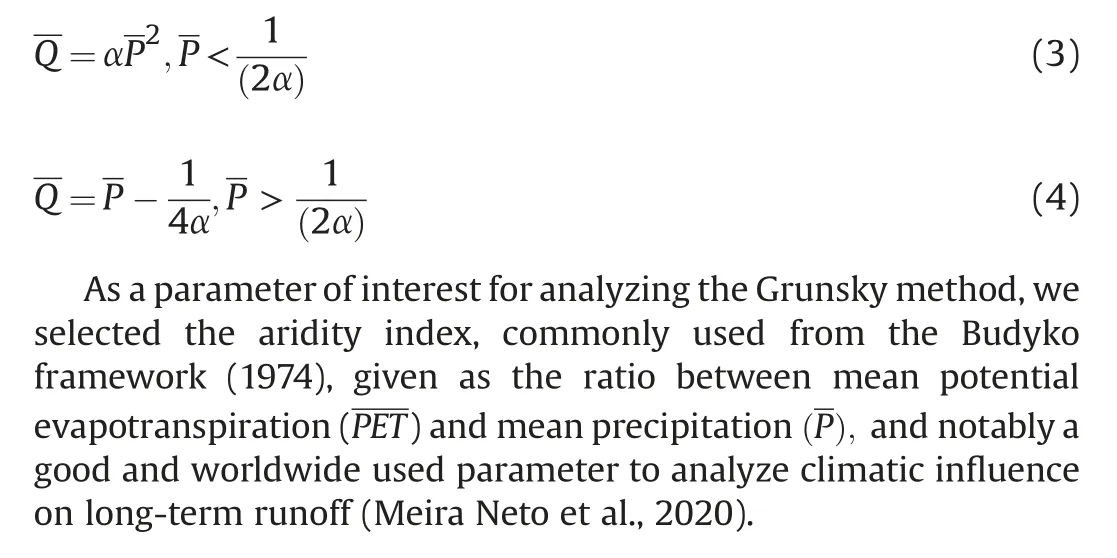
Through Grunsky's analysis(1908,1915), a generalized method to correlate the annual runoff and the annual precipitation resulted in Equations (3) and (4) (Santos & Hawkins, 2011), where α is a coefficient (mm-1) used for this generalization.The generalized equation was applied to California, the South of France, and Portugal, characterized by the Mediterranean climate, with dry summers and wet winters (Santos & Hawkins, 2011).The good fit for Mediterranean catchments arises interest in the study of other types of climates.The rainfall-runoff relationships for varying values of α are presented in Supplementary Material(Fig.S1).As a matter of interest, according to the generalized Grunsky method(Equations (3) and (4)), a negative α value is only possible when runoff is higher than precipitation.On the contrary,when runoff is higher than precipitation,the method does not lead exclusively to a negative α value.Since catchments with Qobs>Pobswere excluded,there are no negative α coefficients in the analysis.
2.3.Computing the α coefficient for interannual and monthly temporal scales on a local scale
According to the Grunsky method,the α coefficient is calculated fromQ and P.As the generalized formula consists of a system of two equations, two values of α are calculated, and the chosen α would be the one that satisfies the system.Nevertheless,the work applied the proposed framework considering a long-term temporal scale, obtaining, therefore, a single α value.In contrast, we evaluated the performance of the Grunsky method on two temporal scales:interannual and monthly.However,in this case,we obtained α values for month and year.Therefore, to keep the consistency with the original framework, for each evaluated temporal scale(interannual and monthly),we chose a single α coefficient that best represents the streamflow in each catchment by maintaining the generalized equation but using values of runoff and precipitation different from the long-termQ and P.
We evaluate three different approaches to obtain this unique α coefficient on a local scale, i.e., one α for each catchment: (i) the mean α among a 30-year series of α values;(ii)the median α among a 30-year series of α values;and the α that presented the Minimum Mean Squared Error (MMSE) between predicted annual runoff(Qpred)and observed annual runoff(Qobs).For the last one,to have more values to make the predictions,and since the most important is to obtain the MMSE value,we used α values from the two sides of Equations (3) and (4).To evaluate the best method to calculate α(mean, median, and MMSE), we compared their Kling-Gupta Efficiency(KGE)(Gupta et al.,2009)coefficient's Empirical Cumulative Distribution Function (ECDF) curves for both evaluated temporal scales.The KGE was computed considering the runoff estimated through one of the three methods to define α and the observed runoff.
To evaluate the prediction performance of the Grunsky method,we applied the equations considering the selected α coefficient(using one of the three proposed approaches)from each catchment and the observed annual precipitation.We then compared estimated and observed streamflow values for both interannual and monthly temporal scales.To evaluate the model performance, we used four widely used statistical metrics: the coefficient of determination(R2),the KGE,the Percent Bias(PBIAS),and the Root Mean Square Error (RMSE).As a matter of interest, R2and KGE values close to 1 represent better model performance,positive(negative)PBIAS indicates overestimation (underestimation) in predictions,and lower RMSE values indicate reduced errors.
2.4.Regionalization of α values
Calculating the α coefficients for each one of the 716 gauged basins would not be the final goal of this study, but a first step for the analysis since we seek to predict streamflow in ungauged basins.After the computation of α,we look for the best classification method to cluster the catchments according to their characteristics.From this cluster classification, it would be possible to define an α coefficient for each group, which, in turn, can be used to predict streamflow fluxes at ungauged basins belonging to the respective group.Prediction in Ungauged Basins passes by a reliable regionalization approach considering multi-criteria analysis (Pool et al.,2021).
To investigate the performance of the regionalization of the α coefficient across Brazil, we used six hydrologically similar groups proposed by Almagro (2021).To define these six hydrological groups, the author used hydrological signatures and attributes of catchments from the CABra dataset and then employed a cluster analysis along with principal component analysis and a random forest algorithm.The catchments were grouped based on their hydrological similarities and the dominant processes and their driving attributes were investigated.The hydrological groups are:“Non-seasonal”, “Dry”, “Rainforest”, “Savannah”, “Extremely-dry”,and“Extremely-wet”catchments(Fig.1).We chose to use these six hydrological groups for the regionalization framework because they can better represent the hydrological similarities than other geographical, climate, or ecosystem groups (Almagro, 2021).
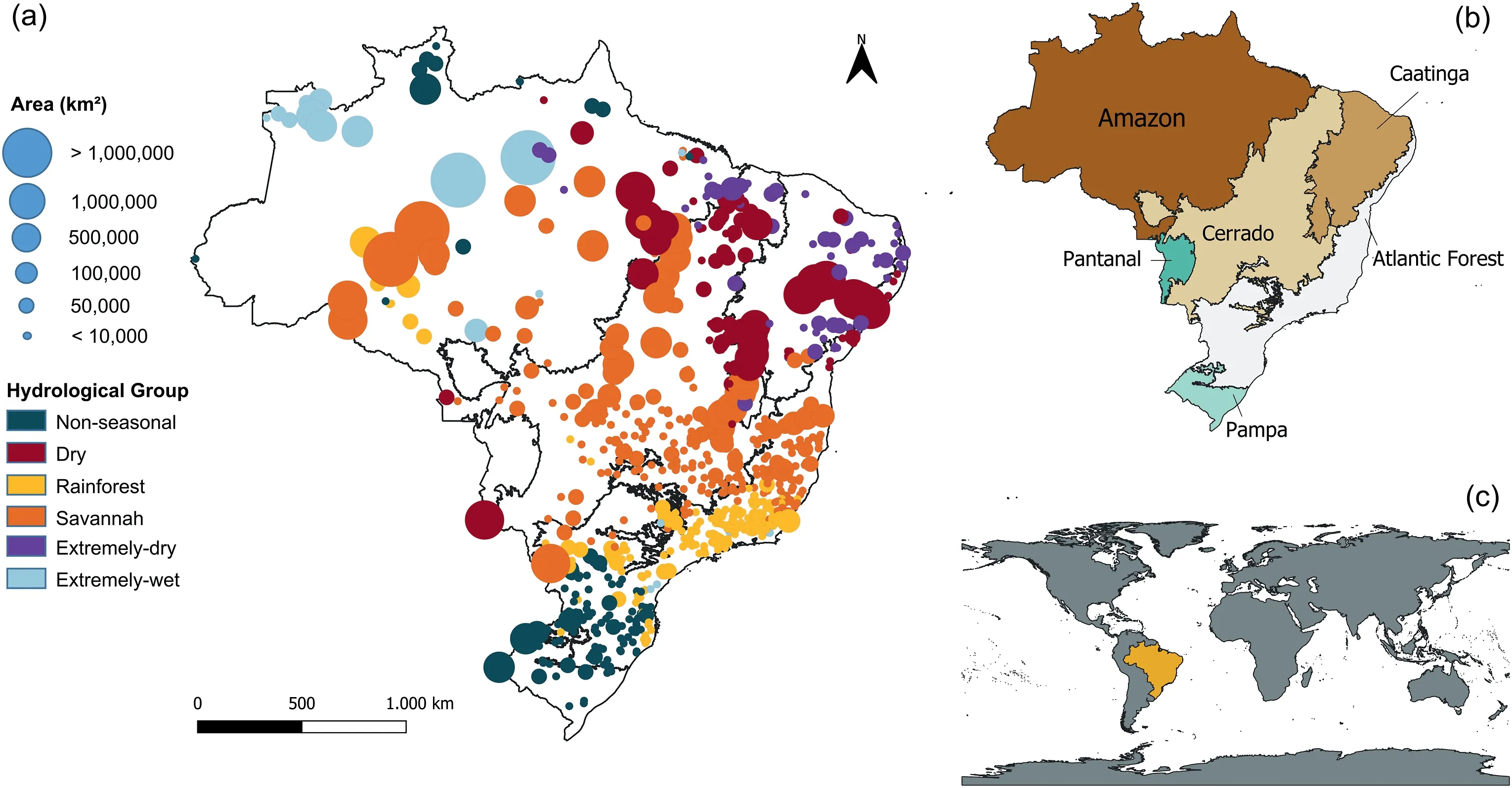
Fig.1.Maps of the spatial distribution of a) each catchment by area and hydrological group over the territory; b) the six Brazilian Biomes (Amazon, Atlantic Forest, Cerrado,Caatinga, Pampa, and Pantanal); and c) Brazil, in yellow, on the world map.
Group 1 (Non-seasonal) presents high values of mean streamflow,with no clear relation between precipitation and temperature throughout the year, with no definitive division between wet and dry seasons.The catchments are located mainly in the South region,with Pampa, Atlantic Forest biomes, and some in the Amazon biome.Group 2 (“Dry”), located mainly in Cerrado biome in the region between Amazon and Caatinga biomes, has well-defined rainy and dry seasons, with the highest temperatures of all groups (20°C-32°C).The catchment's aridity index (the ratio between mean-annual potential evapotranspiration and meanannual precipitation) has a great variance and low values of mean precipitation.Group 3(Rainforest)is located mainly in the Atlantic Forest biome region, with high amounts of precipitation, and a well-defined rainy season, which coincides with the highest temperatures of summer in the region.Group 4 (Savannah) refers to catchments that present savannah characteristics and is located mainly in the Cerrado biome.The vegetation is composed basically of grass and forest,with an aridity index varying from 1 to 2.Group 5(Extremely-dry),located in the Caatinga biome,is covered mainly by grass and shrubs, showing high values of aridity index.This group is different from Group 2(Dry)because of its non-perennial streams.Finally, Group 6 (Extremely-wet) presents the highest values of precipitation and streamflow.The catchments are located in the Amazon and Atlantic Forest biomes and are covered mainly by forests.
To evaluate the performance of Grunsky's framework to predict runoff in ungauged basins, we conducted the following regionalization framework:(i)First,for each catchment of each hydrological group, we computed a median α value using the “leave one out”cross-validation approach.That is,the α of a specific catchment was computed considering the median α from all the other catchments of the same group, except itself.This step is fundamental to preserving independence in the determination of α.Moreover,we use the MMSE value from each catchment as it obtained the best performance among the three evaluated methods(see Results section 3.2).(ii)Then,using the Grunsky method and the median α of step(i),we estimated the runoff for the 716 catchments.(iii)Finally,we evaluated the performance of the regionalized Grunsky method to estimate catchments'runoff through R2,RMSE,and KGE values.We then repeated the same process for each month,on a monthly scale.Here we present a schematic view of the analysis method (Fig.2).
3.Results and discussion
The results are presented in four steps: (i) We first assess the relationship between observed annual runoff (Qobs) and precipitation (Pobs) with the Grunsky method and (ii) choose the best α value for each catchment in both interannual and monthly temporal scales.(iii) Then we evaluate the Grunsky's framework for each time scale on local analysis,catchment by catchment;and(iv)finally, we assess the performance of the proposed regionalization method to compute interannual and monthly streamflow across Brazil.
3.1.Relations between runoff, precipitation and the Grunsky equation
Fig.3 shows a scatter plot between Pobsand Qobsfor each year of the 30-year time series of the 716 evaluated catchments, colored according to their aridity index computed annually, and the Grunsky method plots for multiple α values.We noted that the relation between Pobsand Qobsfollows, in general, the Grunsky Generalized curve(Equations(3)and(4))and fits well for both low and high α values, indicating the Grunsky framework is able to capture the inter-catchment and annual rainfall-runoff relationship variability.However, when looking at the aridity index values, we note lower dispersion of the Grunsky curve for aridest catchments,due to the high initial abstraction during rain events in dry catchments(de Figueiredo et al.,2016).The highest aridity index values occur for catchments with lower Pobsamounts, and they show a better fit to the Grunsky curve than for lower values of aridity index when Pobspresents higher values.These results were somehow expected since the method was proposed and has already been applied to Mediterranean catchments, which are generally drier than most of the climate types in Brazil (Spinoni et al., 2015).
The observed scatter values agree with the behavior of Grunsky generalized method functions, with α values ranging from 0.0002 to 0.0004.Even the catchments with higher long-term mean annual rainfall (P > 2000 mm year-1) fall inside the interval between the theoretical curves.Our results corroborate with those reported by Santos and Hawkins (2011), which presented α values from 0.00009 to 0.00043 mm-1,with the highest Pobs=2770.1 mm.We also noted that values tend to be sparse for precipitations higher than 2000 mm year-1, as observed previously.
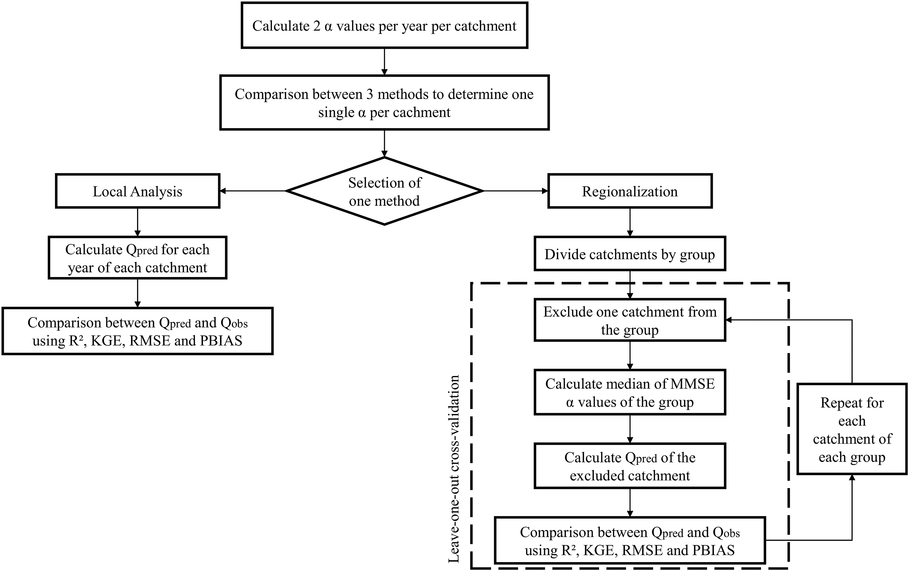
Fig.2.Schematic view of the analysis method.
3.2.Choosing the best method to define a single α for each catchment
We analyzed the rainfall-runoff relations for the interannual and monthly scales, considering, however, a single α value for each catchment, calculated by the three different methods described in Section 2.3 (mean, median, and MMSE).To better visualize de variability of α values calculated from the 30-year series, we presented them in Supplementary Material(Fig.S2),separated by the different hydrological groups in both interannual and monthly scales.
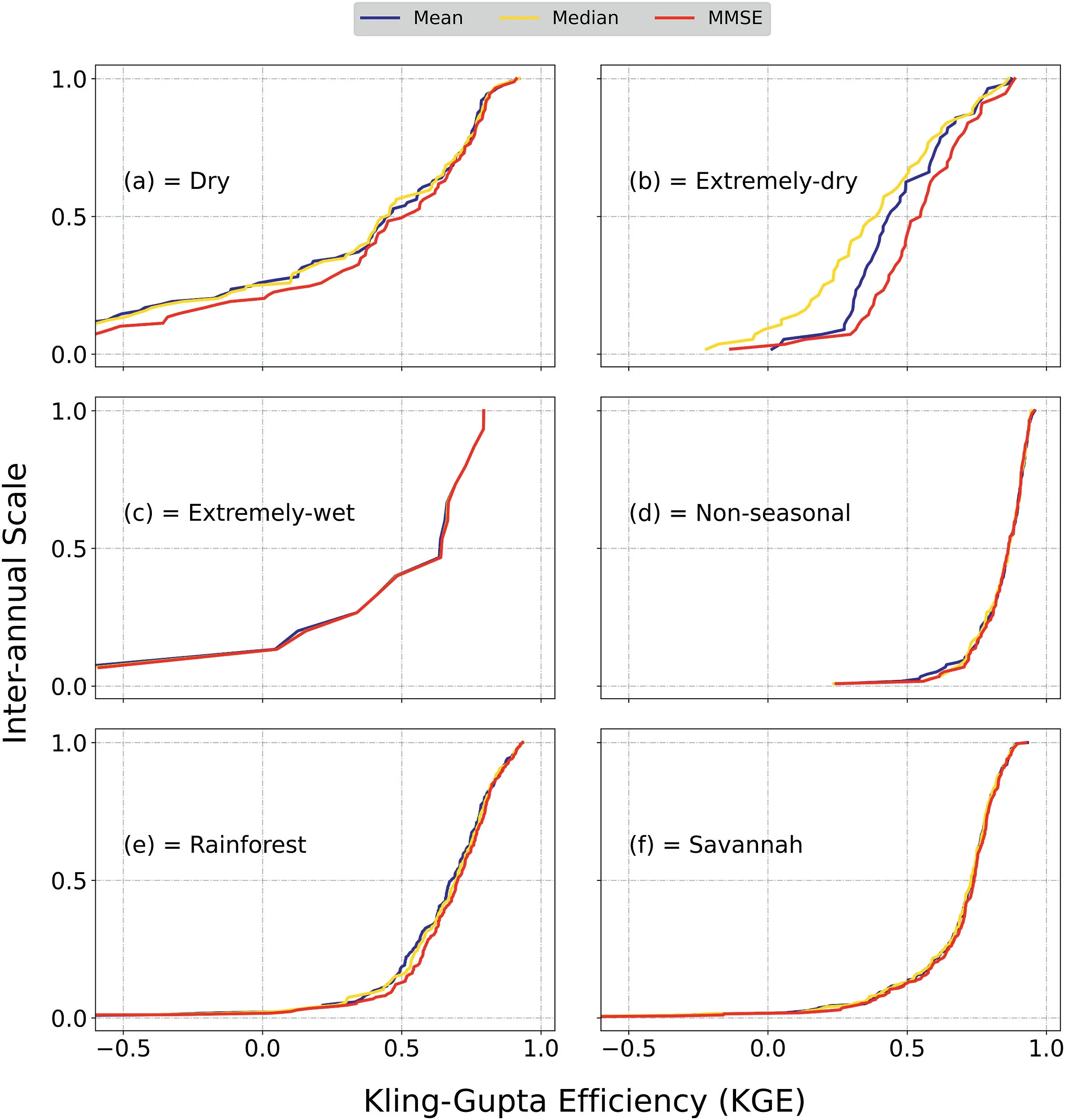
Fig.4.Cumulative Distribution Function(CDF)curves comparing KGE values for each method for determining α coefficient on an interannual scale,for hydrological groups a)Dry,b)Extremely-dry, c) Extremely-wet, d) Non-seasonal, e) Rainforest and f) Savannah.
From the interannual analysis, it is evident that the behavior of the α coefficient changes according to each hydrological group.The difference between the boxplots of the three evaluated approaches(mean,median,and MMSE)was not so remarkable.Nevertheless,it is possible to note that the α values estimated through the mean approach exhibited a larger variability.Interestingly, although the MMSE method involves more complex calculations to determine α,using linear regressions between predicted and observed runoff to define the α that minimizes Minimum Square Error (MSE), it obtained a very similar variability to the median approach.This does not hold for the monthly temporal scale.In this case, the MMSE approach showed the lowest variations.As expected,α is higher for wetter catchments and lower for drier catchments.Dry and Extremely-dry groups show the lowest MMSE α values for all methods.These values are coherent to scatter plots per hydrological group on Supplementary Material (Fig.S3), where there's a higher density of points near the curve for α = 0.0001 for these drier groups.
The α values obtained for each month by using the three evaluated approaches were presented in Supplementary Material(Fig.S4).We found that the α coefficient presents a higher range in May,June,July,and August,the driest months of the year in Brazil,which was expected since, during this period of the year, a great part of Brazilian territory is affected by climatic instability and higher variability in the rainfall-runoff relation (Silva & Sim˜oes,2014; Zhang et al., 2018).For the Caatinga biome (Dry and Extremely-dry groups), Pinheiro et al.(2016)found that soil water content has a stronger influence on evapotranspiration and air temperature during the June-September and December-January periods, which increases the uncertainty of the Grunsky method by adding more variance to hydrological processes.
Differently from mean values,median α shows a lower scatter in all months, especially in May, though it still presents high variability in June, July, and August.We observed that the α MMSE value resulted in a great decrease in α dispersion,given the purpose of this method to determine an α value that minimizes errors for each catchment, with only the months June and July having a higher variability in α values.These variations were higher than that found in the same months for the median and mean values.We also noted that, on a monthly scale, α values tend to be approximately one order of magnitude higher than that obtained on an annual scale.This fact was already expected since annual precipitation is divided by the 12 months of the year,and by Equations(3)and (4),α is proportionally inverse to precipitation.
The MMSE α values present better results of KGE's ECDF for all groups, especially for Dry and Extremely-dry groups, where the difference from the other methods is more clear on an interannual scale (Fig.4).This result contradicts the already indicated in the scatter plot of Fig.3, which presented the best results from drier catchments,while Fig.4 shows that the best performances are from the Non-seasonal, Rainforest, and Savannah groups.Whereas KGE assumes mainly values from 0 to 1 in some groups, a part of catchments presents negative values, which does not imply a bad simulation,since KGE values higher than-0.41 still indicate a good performance compared to a mean flow reference (Knoben et al.,2019).The MMSE α values spatialized for each studied catchment,are found in Supplementary Material (Fig.S5).
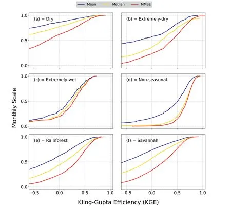
Fig.5.Cumulative Distribution Function (CDF) curves comparing KGE values for each method for determining α value on a monthly scale, for hydrological groups a) Dry, b)Extremely-dry, c) Extremely-wet, d) Non-seasonal, e) Rainforest and f) Savannah.
On a monthly scale (Fig.5), it is more evident that MMSE α values, in general, for all groups, present better results than mean and median values.Among the groups, the best results are for the Non-seasonal group,with a great percentage of KGE>0.50.The Dry group presents more than 50%of values below 0,indicating worse predictions.As the MMSE presented a better performance in runoff prediction than the other approaches evaluated for interannual and monthly temporal scales, we used α values obtained by the MMSE in our study, for local and regionalized analysis.For details of boxplots of Monthly Observed Precipitation(mm)and Runoff(mm)for each hydrological group(see Supplementary Material, Figs.S6,S7, and S8).
The difference in performance on different groups and time scales comes from the non-linearity of arid catchments’ behavior,especially for hydrological extremes, which might affect the intraannual behavior more than interannual and long-term runoff.On the other hand, more humid catchments, given their more (relative) linear behavior, tend to have better performance (Parajka et al.,2013; Salinas et al., 2013).
3.3.Local performance of α values
The predicted runoff was calculated then by Grunsky Equation using the MMSE α value for each catchment on an interannual and monthly scale.The correlation between Predicted Runoff and Observed Runoff was then evaluated using metrics such as R2,KGE,relative RMSE (absolute RMSE divided by mean runoff of each group),and Percentage Bias (PBIAS).
3.3.1.Interannual scale
Fig.6 illustrates the relations between predicted and observed annual runoff for each group, colored by point density with the number of neighboring points.All groups present R2higher than 0.80, considered a satisfactory result, especially for the Dry group,which shows R2= 0.93.RMSE is higher for Extremely-dry (48.3%)group,and smaller for Extremely-wet(13.1%),Non-Seasonal(18.3%)groups,also corroborating with the previous analysis from Section 3.1, as smaller RMSE indicates a better correlation.KGE shows values close to 1 in almost all groups,indicating a high correlation.Dry, Savannah, and Extremely-wet groups present higher KGE(0.93, 0.90, and 0.90, respectively).The predictions show higher KGE values than other studies, such as Gao et al.(2021), that predicted mean annual runoff in 35 catchments in the United States with the use of a water balance model calculated from Budyko-type equations and spatial distribution models for soil data,resulting in R2= 0.76.
The higher correlations found in the present study may indicate a constant behavior of each catchment during the 30-year series,generating an α value that well represents the catchment.In addition, it can be noted that catchment characteristics according to each group may influence α for a better correlation,although it is not possible to well differentiate the performance between drier and wetter groups.It is interesting to note that even the Nonseasonal group presented a KGE = 0.90 even though this group does not present a very defined behavior of seasonality between water and energy availability(Almagro,2021),with a great variety of hydrologic characteristics of catchments.
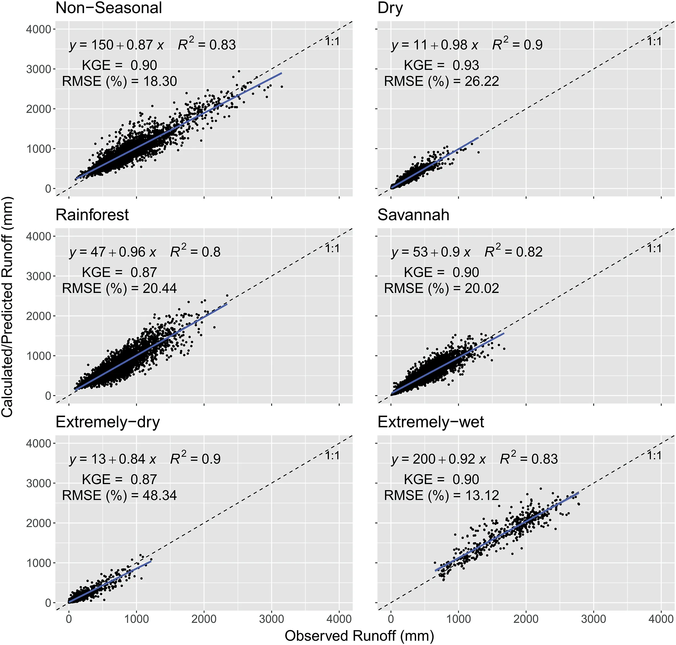
Fig.6.Scatter plot with observed annual runoff versus predicted annual runoff from MMSE α value for each catchment during the 30-year series from the 716 CABra catchments,divided by groups.Values are in mm and colored by the number of neighbors for each point.
To understand the correlation between predicted and observed runoff during the 30-year series, KGE and PBIAS values for each catchment were spatialized within the Brazilian territory,as shown in Supplementary Material (Fig.S9).The higher values of KGE for the catchments are mainly located where there are the groups with higher values of precipitations (Non-seasonal in the south region,Rainforest in the southeast, and Extremely-wet in the northwest).Also,the Dry and Extremely-dry groups present values closer to 0,indicating a relatively lower correlation according to KGE.The highest positive PBIAS values (>20%) correspond to the northeast region (Dry and Extremely-dry groups), indicating an overestimation of the model.The other regions of the territory mainly present negative PBIAS,indicating an underestimation of Qobs.The PBIAS values range mostly from -5 to 5%.Also, as discussed for KGE,a lower value of PBIAS was found for the wettest catchments.One should remember that these values refer to one α value for each catchment, corresponding to the MMSE for each catchment.The regionalization prediction would be evaluated by using a single α for each hydrological group, discussed in Section 3.4.
3.3.2.Monthly scale
At the monthly scale, we calculated the MMSE α value for each catchment,and the spatialized values according to each month are on the Supplementary Material (Fig.S10).It was observed that in the Southeast region (Non-seasonal, Savannah, and Rainforest groups),the drier months(i.e.,from May to August,especially June and July) correspond to the lowest KGE values (Fig.7).During the other months, KGE values are in general higher than 0.50, which indicates a good model prediction, especially for wetter months.The hydrological modeling performance variability between Brazilian climate regions was also observed on a daily analysis by Almagro et al.(2021), that pointed out KGE ≤0.50 for catchments with not well-defined wet and dry seasons.Further, Siqueira et al.(2018), obtained KGE <0.40 for regions with arid and semiarid climates, and KGE ≥0.60 for wetter climate catchments in South America.
PBIAS between Predicted Runoff and Observed Runoff was calculated for all months, and the results are shown in Supplementary Material (Fig.S11).The maps indicate a prevalence of negative PBIAS,implying an underestimation in MMSE predictions,i.e., the predicted runoff is lower than the observed one.The months with the highest bias differ between regions, being the Southeast region with the highest biases, mainly from January to March,and August to October.The lowest biases are observed in the North region(Extremely-wet and part of the Savannah group),with the highest biases from August to October.
3.4.Regionalization of α values
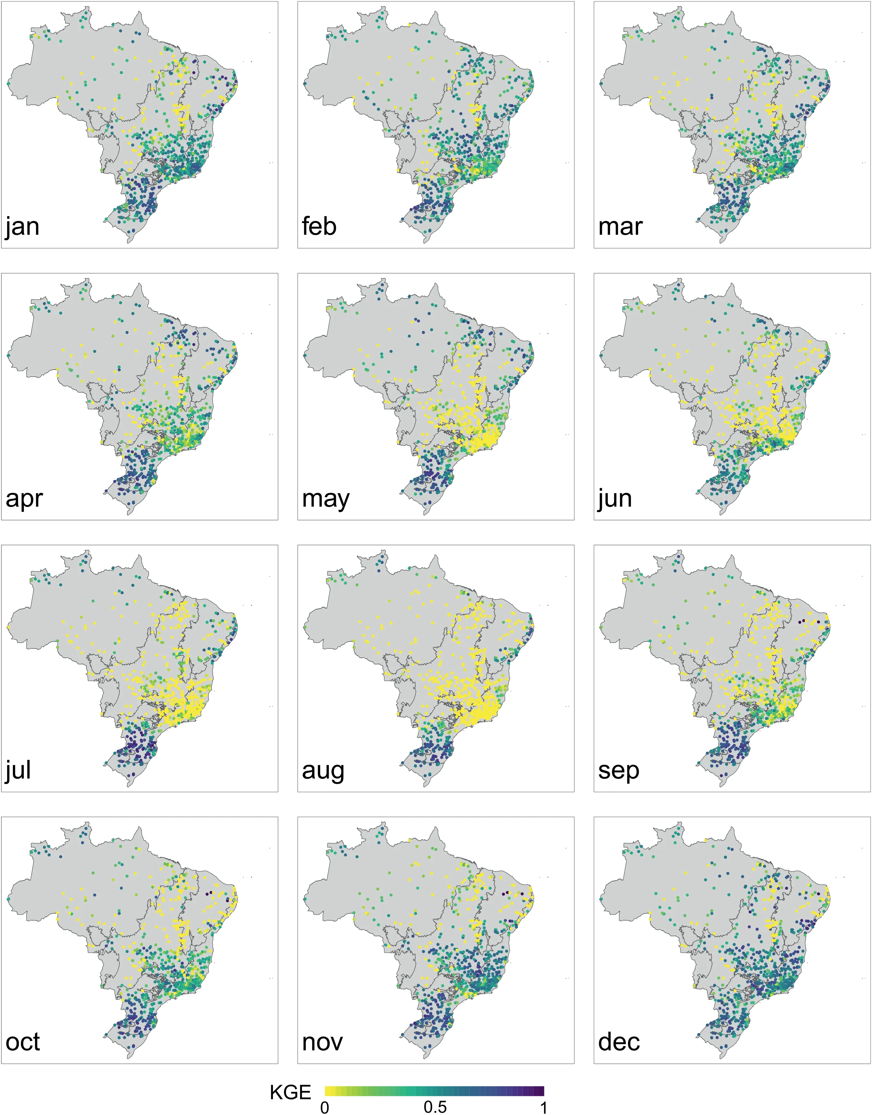
Fig.7.Maps of KGE from MMSE α value for each group for each month, from January (top left) to December (bottom right).
It is important to analyze the α coefficient according to catchment characteristics and to define a proper clustering proposal that can be used for predictions on ungauged basins.The clustering proposal analyzed was the hydrological group division (Almagro,2021), on an interannual and monthly scale.Results for the regionalization approach are described below.
3.4.1.Interannual scale
We evaluate the use of six α values to predict runoff across Brazil, calculated from the median of the MMSE α values of the catchment belonging to the groups (Table 1).The correlation between Predicted Annual Runoff and Observed Annual Runoff was then evaluated by leave-one-out validation, using metrics such as R2, KGE, RMSE,and PBIAS, as described in Section 2.4.
Fig.8 illustrates the relations between predicted and observed annual runoff for each group, colored by the scatter density withthe number of neighboring points.As expected, the predictions present a lower correlation than local analysis when a single α value is used for each hydrological group.The group that did not perform so well is the Extremely-dry group (R2= 0.67 and KGE = 0.60), and the best one is the Non-seasonal (R2= 0.74 and KGE = 0.84).Despite worse prediction indicators for each group,KGE and R2were higher than 0.60 and 0.49, respectively, for all groups, highlighting the good performance of the method on an interannual scale, considering all years of a series within one catchment.RMSE is higher for Extremely-dry (89%) and Dry (51%)groups, and smaller for Non-seasonal (22%) and Extremely-wet(16%).

Table 1 Median of MMSE α value (mm-1) of each hydrological group, for an interannual scale.
3.4.2.Monthly scale
The regionalization on a monthly scale was done by assuming one α coefficient for each group and month,from the median values from the catchments.Fig.9 shows the boxplots of KGE values for the 12 months divided by each group.These α values and the boxplots of PBIAS values are exhibited in the Supplementary Material (Table S2 and Fig.S12, respectively).
The groups with the lowest values of PBIAS and highest values of KGE are Non-seasonal and Extremely-wet, given a more constant rainfall behavior on an intra-annual scale (Almagro, 2021).The worse performance was the Dry group,with median monthly KGE<0 for all months, and PBIAS >100% from June to August.The regionalization for a monthly scale appears to have worse results than the interannual scale for all groups,indicating the influence of interannual and intra-annual behavior of streamflow on the method's performance.The results appear to be similar to the predictions by Arheimer et al.,2020,which showed relatively good results in Brazilian North region catchments when predicting monthly runoff, with median monthly KGE >0.60, and worse performance in the North-east region, with KGE < -1,00.Dry and Extremely-dry groups might have higher variance on an intraannual scale due to the influence of soil water content, and high rates of evapotranspiration (Pinheiro et al., 2016).
For a seasonal analysis,we combined the monthly regionalized predictions into the four seasons of the year,namely(i)December,January,and February(DJF),(ii)March,April,and May(MAM),(iii)June, July, and August (JJA), and (iv) September, October, and November(SON).The results reinforce the higher variability of the driest season(JJA),with a KGE=0.36.The wetter seasons presented similar results, with KGE = 0.73 (SON), KGE = 0.66 (DJF), and KGE = 0.62 (MAM) (See Fig.S13).
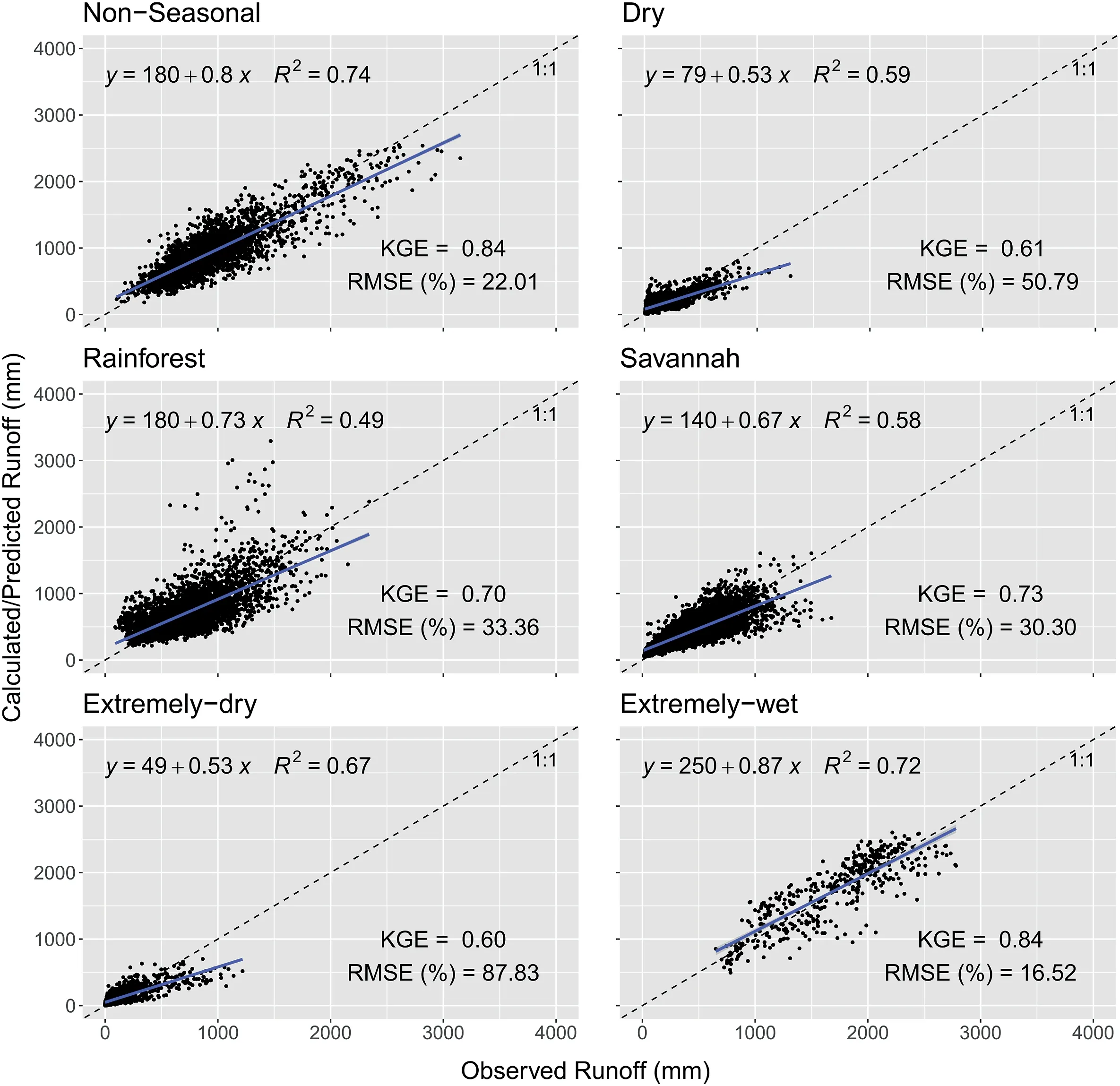
Fig.8.Scatter plot with observed annual runoff versus predicted annual runoff from median MMSE α value for each group during the 30-year series from the 716 CABra catchments,divided by groups.Values are in mm and colored by the number of neighbors for each point.
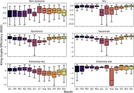
Fig.9.Boxplot with KGE from regionalized monthly runoff prediction for each month and group from the 716 CABra catchments.
4.Limitations and broader implications
This paper has demonstrated the usefulness of the Grunsky method on an annual and monthly scale, especially for wetter catchments.Broader studies are required for the performance improvement in drier catchments, such as consideration of the hydrological balance and inter-catchment groundwater fluxes, as proposed by Liu et al.(2020)and Schwamback et al.(2022).
The analysis methods employed, due to their relative ease of application, have great replication capacity.That is, they may be used for a large database of hydrographic basins,as is the case with CABra,and can be updated in the future,as needed.Further studies may complement and enrich the topic discussion through the adaptation of the methods already described,or further analysis of other characteristics of hydrographic basins since the database has a great variety of data.Through the CABra database,especially the values of precipitation and flow in different time scales, it is possible to analyze the influence of environmental factors on runoff response to precipitation.
Regionalization is an important tool for the estimation of water availability in poorly or ungauged catchments (Athira et al., 2016),and contributes to different water uses (Agarwal et al., 2016; Bork et al., 2021), mainly in developing countries where hydrological data are scarce(Beskow et al.,2016).In Brazil,legislation on water resources allows each state to determine its values of reference for granting water use privileges (Honˊorio et al., 2020).In several Brazilian states, the reference environmental flow is the Q95permanence flow,which guarantees that the flow of a determined river equals or surpasses this value 95%of the time(ANA,2007;Piol et al., 2019).Broader studies might be needed seeking the performance evaluation of the Grunsky method for practical purposes such as predicting permanence flow curves for different water uses.
5.Conclusions
This study aims to predict runoff in ungauged basins from values of precipitation and the α coefficient applied to a simple and easyto-use equation.Considering the practical use of the method, our study presents a reliable alternative to more complex methods to calculate runoff from very few parameters.We expanded Grunsky method usage from Mediterranean to tropical climate basins in Brazil,which might be an important tool for future studies,support fast decision-making processes, and hydraulic projects, from irrigation to dam constructions, and generate permanence flows for licensing projects.From this analysis, some conclusions deserve special attention and are described below.
Results could show that the Grunsky method can be applicable for Brazilian catchments, having a good fit, especially for Nonseasonal and Extremely-wet catchments on annual and monthly scales, showing less variability in both interannual and intraannual scales.The best method to obtain α for each catchment is the MMSE method, with suitable results for annual and monthly analysis, for all hydrological groups.
In the regionalized approach, the Kling-Gupta Efficiency (KGE)ranges from 0.60 to 0.84 when examined on an interannual scale.Furthermore, we observed favorable KGE values at a monthly resolution, with over 22% of catchments exhibiting KGE values exceeding 0.50.The Non-seasonal and Extremely-wet groups demonstrated the highest performance, while the Dry group exhibited the poorest performance.Considering the usage of each approach, the regionalization method, using a single α coefficient for each hydrological group, has a wider use for ungauged basins,although a local analysis might be convenient for analysis on poorly gauged catchments since it shows a better performance.
Declaration of competing interest
The authors declare that they have no known competing financial interests or personal relationships that could have appeared to influence the work reported in this paper.
Acknowledgments
We would like to thank Prof.Richard H.Hawkins for introducing us to the Grunsky studies and theories.The authors acknowledge the Graduate Program in Hydraulic Engineering and Sanitation -PPGSHS (USP-EESC) and Graduate Program in Environmental Technologies - PPGTA (UFMS-FAENG) for the scientific support.This study was supported by grants from the Coordination for the Improvement of Higher Education Personnel (CAPES) - Finance Code 001 and CAPES PrInt,the Ministry of Science,Technology,and Innovation (MCTI) and National Council for Scientific and Technological Development (CNPq) (grants numbers 441289/2017-7 and 309752/2020-5), and São Paulo Research Support Foundation(FAPESP,grants numbers 2015/03806-1,2019/24292-7,and 2020/08140-0), Foundation for the Development of Education, Science and Technology of the State of Mato Grosso do Sul - FUNDECT(grant number 71/032.795/2022).
Appendix A.Supplementary data
Supplementary data to this article can be found online at https://doi.org/10.1016/j.iswcr.2023.06.004.
 International Soil and Water Conservation Research2023年4期
- International Soil and Water Conservation Research的其它文章
- Legacy earthen berms influence vegetation and hydrologic complexity in the Altar Valley, Arizona
- Long-term trends of precipitation and erosivity over Northeast China during 1961-2020
- Atlas of precipitation extremes for South America and Africa based on depth-duration-frequency relationships in a stochastic weather generator dataset
- Towards a better understanding of pathways of multiple co-occurring erosion processes on global cropland
- Saturation-excess overland flow in the European loess belt: An underestimated process?
- Calibration,validation,and evaluation of the Water Erosion Prediction Project (WEPP) model for hillslopes with natural runoff plot data
