Monocular Depth Estimation with Sharp Boundary
Xin Yang,Qingling Chang,Shiting Xu,Xinlin Liu and Yan Cui,,*
1Faculty of Intelligent Manufacturing,Wuyi University,Jiangmen,529000,China
2China-Germany(Jiangmen)Artificial Intelligence Institute,Jiangmen,529000,China
3Zhuhai 4DAGE Network Technology,Zhuhai,519000,China
ABSTRACT Monocular depth estimation is the basic task in computer vision. Its accuracy has tremendous improvement in the decade with the development of deep learning.However,the blurry boundary in the depth map is a serious problem.Researchers find that the blurry boundary is mainly caused by two factors.First,the low-level features,containing boundary and structure information, may be lost in deep networks during the convolution process.Second,the model ignores the errors introduced by the boundary area due to the few portions of the boundary area in the whole area,during the backpropagation.Focusing on the factors mentioned above.Two countermeasures are proposed to mitigate the boundary blur problem.Firstly,we design a scene understanding module and scale transform module to build a lightweight fuse feature pyramid,which can deal with low-level feature loss effectively.Secondly,we propose a boundary-aware depth loss function to pay attention to the effects of the boundary’s depth value.Extensive experiments show that our method can predict the depth maps with clearer boundaries,and the performance of the depth accuracy based on NYU-Depth V2,SUN RGB-D,and iBims-1 are competitive.
KEYWORDS Monocular depth estimation; object boundary; blurry boundary; scene global information; feature fusion; scale transform;boundary aware
1 Introduction
Monocular depth estimation is a base vision task in computer vision. It is widely used in autonomous driving, height measurement, SLAM (Simultaneous Localization and Mapping), AR(Augmented Reality),etc.Monocular depth estimation is denser and more low-cost than traditional cost sensors to obtain depth directly.Furthermore,it has the advantages of low price,rich information acquisition content,and small size compared with the binocular image which is limited by the baseline length resulting in a poor match between the volume of the equipment and the vehicle platform.So,estimating depth information based on monocular cameras has become one of the research hotspots in computer vision.Monocular depth estimation refers to transforming a 2D RGB image into a 2.5D depth map,which relies on the“Shape From X”methods to obtain the scene depth information from an RGB image.Monocular depth estimation is an ill-posed problem because a single image lacks the geometrical information required to infer the depth from the image. Compared with the traditional methods[1,2],etc.,that use the cues designed artificially,learning-based monocular depth estimation methods use Convolutional Neural Networks(CNNs)to extract features from images instead of the artificial cues and build the mapping between features and depth. Eigen et al. [3] proposed the first monocular depth estimation method based on deep learning,which showed a surprising performance than pre-works [1,2]. Then, a lot of excellent works based on deep learning were proposed such as[4-14]. However, monocular depth estimation methods have still suffered from the boundary blur challenge, especially in indoor scenes which have complex scene structures and many objects. Fig.1 shows the estimation depth results from existing works in indoor scenes.From the red box in Fig.1,we can see that Hu et al. [15] have a significant improvement in depth accuracy compared with Eigen et al. [3], furthermore, the object structure in the depth maps is more clear. But there is still an obvious boundary blur phenomenon,especially in the complex object structure and some objects are given a wrong depth value that is close to the background.The blurry boundary not only increases predicting errors in the depth estimation but also causes the“flying pixels”[16].Some cases of“flying pixels”in the point cloud can be seen in Fig.2.Looking the Fig.2,the first group shows that the point clouds from Hu et al. [15], and Chen et al. [17] have serious “flying pixels”in the human head, the point clouds are discontinuous. In the second group, the screens are wrapped. The projected point clouds from depth maps are discontinuous, especially in the object boundary. The blurry boundary leads the depth values of pixels from boundary and non-boundary are different and the pixels with different depth values will be projected to different planes,which lead the boundary and non-boundary area in the same object to be separated like Fig.2. Studies find that the boundary blur problem is mainly brought about by two factors in the CNNs frameworks.Firstly,the loss of low-level features in the encoding phase, the low-level feature includes scene structure and object information, which lead the depth maps to unclear and blurry object boundary.But the deep network is needed to improve the spatial expression ability and receptive field of the features due to the deeper network can extract the high-level and abstract information of images such as depth information.Secondly,the“boundary smoothing”during model training(Boundary smoothing:the loss caused by boundary area is ignored during model training,due to the boundary area occupying a little proportion.Although the gradient of boundary is larger,it causes little loss in training.The model processing the boundary as the nonboundary with a small gradient leads to the boundary not sharp and clear enough,like the methods[15,17] in Fig.1) In this paper, we propose two solutions for these two impact factors, respectively.Firstly, to mitigate the low-level information loss, we propose a Scene Understanding module (SU)and a Scale Transform module(ST).Secondly,to solve the problem caused by“boundary smoothing”,we pay attention to the loss introduced by the boundary area and design a novel depth loss function Boundary Aware Depth loss(BAD).
SU and ST.The multi-scale feature fusion is an effective method to deal with low-level feature loss.The Fuse Feature Pyramid(FFP)is a usual method to aggregate different scales feature,such as Chen et al.[17],and Yang et al.[18],but these models have a lot of parameters due to sampling the features too many times during building the FFP.To reduce the parameters,SU and ST are designed in this work.SU is used to aggregate all scales feature,extracted from all encode phases,and learn the global scene information which includes rich scene structure and boundary information.Then,ST is used to transform the global scene information to different scales to build the lightweight FFP.The feature in FFP will be connected with each corresponding scale in the decoder.
BAD.BAD will guide the model to focus on the boundary area during model training. BAD introduces boundary weights based on the depth loss function,the weight composed of multi-items to ensure it is useable in most cases.The BAD Will enforce the model to pay attention to the loss caused by the boundary area.
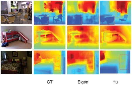
Figure 1: Predicted depth map from other methods. From left to right are the input image, Ground truth,and the predicted from Eigen et al.[3]and Hu et al.[15]

Figure 2: The flying pixels phenomenon in the projected cloud from depth maps. From left to right are input RGB images, ground-truth depth maps, and results of Hu et al. [15], and Chen et al. [17],respectively
Contributions:
1. We propose a Scene Understanding module(SU)to aggregate the multi-scale features of the encoder and learn the global scene information. Furthermore, we design a Scale Transform module (ST) to transform global information to different scales to build a lightweight FFP that deals with the low-level feature effectively.
2. We propose a novel Boundary Aware Depth loss(BAD).BAD introduces a boundary aware weight to the depth loss and guides the model to be aware of these pixels which have high edge gradients.
3. Extensive experimental results show that our model can predict depth maps with clearer boundaries,which can effectively alleviate“flying pixels”and show competitive depth accuracy in the NYU-Depth V2[19],SUN RGB-D[20],and iBims-1 datasets[21].
2 Related Work
Monocular depth estimation is an important task in computer vision. The beginning of the learning-based monocular depth estimation is Eigen et al.[3],which predicted the depth from a single RGB image with CNNs. Eigen et al. [3] showed a great performance over the previous works [1,2].Based on this work, Eigen et al. [4] proposed a universal multi-task framework to predict depth,surface normal,and segments from a single image.After that,the monocular depth estimation made great progress. Some researchers proposed to the fusion of the CRF (Conditional Random Field)and deep learning [22-25]. Combining CRF and CNNs makes up for the problems of CNNs and improves the accuracy of the depth estimation models. In addition, Fu et al. [26-28] proposed the use of classification to deal with monocular depth estimation. They divide the depth interval of the image and solve the pixel interval corresponding to each pixel and use the depth value corresponding to the depth interval to express the depth of each pixel.These works show a great performance in the depth predict,but ignore the structure information in the depth map,which will impact the effects of reconstruction or obstacle detection with point clouds projected from a depth map without or with less structure information.This flaw is fatal,especially in complex scenes such as indoor scenes,which have complicated structures and a mass of objects.Clear object boundary not only improves the accuracy of depth estimation but also keeps the point cloud in great shape,which is conducive to upper-level work such as scene reconstruction and object detection. To deal with the blurry boundary, Hu et al. [15]proposed a fusion model to fuse multi-scale features and proposed a compound loss function to make the boundary clearer.Based on this excellent work,Chen et al.[17]proposed a Fused Feature Pyramid(FFP)and a residual pyramid to predict depth maps.Yang et al.[18]built an FFP and used an ASFF(Adaptively Spatial Feature Fusion)structure[29]to fuse the different scale depth maps to keep the structure information.Although Chen et al.[17]and Yang et al.[18]showed a great performance,their model has a lot of parameters for building the FFP.Based on this work,we propose a SU module to fuse the multi-scale feature, which learns the global scene information. And then use ST module to transform the global scene information to build a more lightweight FFP than pre-works.Furthermore,to predict the depth including clearer object boundary,we propose a novel depth loss BAD to enforce the network to punish the depth error in the boundary field.
3 Methods
In this section, we first introduce the overall framework, and then we describe the Scene Understanding module (SU), the Scale Transform module (ST), and Boundary Aware Depth loss(BAD)in detail successively.
3.1 Overall Framework
A blurry boundary not only introduces errors in depth maps but also causes“flying pixels”in point clouds,to alleviate the boundary blur problem,we design a framework,which is shown in Fig.3,and the detail on the structure is shown in Table 1(H is height,W is width C is the number of channels),to predict the depth maps with a clear boundary. This framework uses the encoder-decoder as the based architecture and selects the SeNet154[30] as the backbone. Besides the base encoder-decoder architecture,we designed the SU module to aggregate all extracted features to learn the scene global information and ST module to transform the global information to different scales.The different scale global information will be sent to each step of the decoder.In the decoder,we use the u-net architecture.The features of the backbone will be compressed to half of the original and participate in the decoding as a skip connection. In the decoder, the decoding results of each layer will be compressed and use bilinear interpolation to the corresponding resolution and participate in the next layer decoding.As shown in Fig.3 and Table 3.In the model training,we propose a novel loss function Boundary Aware Depth loss(BAD)to enforce the model to focus on the object boundary in the training process but not ignore it directly.
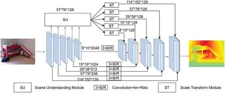
Figure 3:The architecture of our framework.SU is the Scene Understanding module and the ST is the Scale Transform module
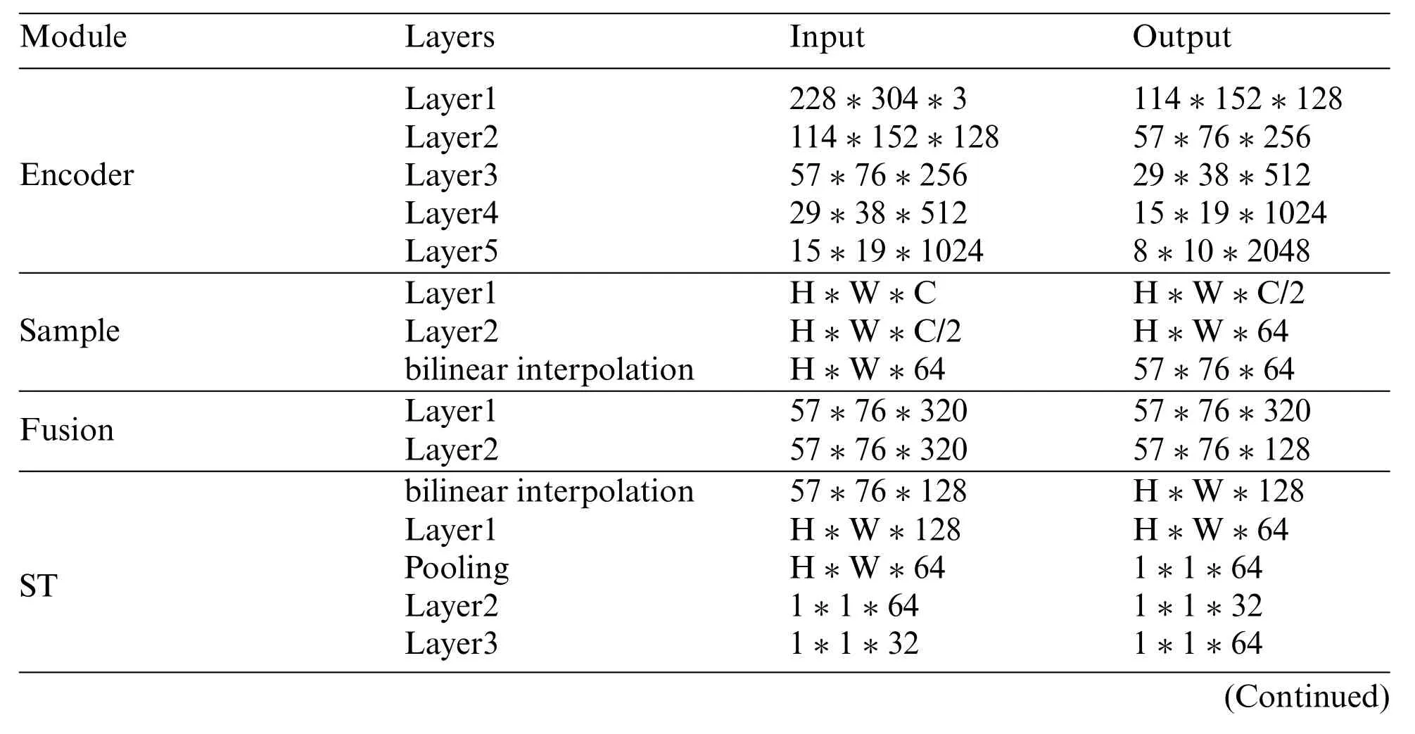
Table 1:Sizes of output features,and input/output channels of each layer when using a SeNet154 as the encoder
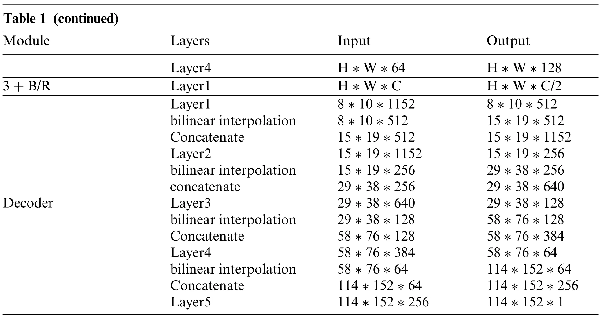
Table 1 (continued)Module Layers Input Output Layer4 H*W*64 H*W*128 3+B/R Layer1 H*W*C H*W*C/2 Decoder Layer1 8*10*1152 8*10*512 bilinear interpolation 8*10*512 15*19*512 Concatenate 15*19*512 15*19*1152 Layer2 15*19*1152 15*19*256 bilinear interpolation 15*19*256 29*38*256 concatenate 29*38*256 29*38*640 Layer3 29*38*640 29*38*128 bilinear interpolation 29*38*128 58*76*128 Concatenate 58*76*128 58*76*384 Layer4 58*76*384 58*76*64 bilinear interpolation 58*76*64 114*152*64 Concatenate 114*152*64 114*152*256 Layer5 114*152*256 114*152*1
3.2 Scene Understanding Module(SU)and Scale Transform Module(ST)
Scene Understanding module(SU).In the deep network,the low-level features are always lost which lead to the blurry boundary.Monocular depth estimation is a dense prediction vision task that needs to use deep CNNs to extract high-level features to establish the mapping between the RGB field and depth field.To deal with this problem,we propose that the SU aggregate and learn the global scene information containing the low-and high-level features.The architecture of SU is illustrated in Fig.4.Firstly, to reduce the model parameter we use two convolution layers with convolution, the kernel size is 3 * 3 to compress these feature maps which are extracted from the backbone to 64 channels.Secondly,we use bilinear interpolation to sample these feature maps to the second scale resolution(57*76).Finally,we concatenate the feature maps and use a fusion layer to fuse these feature maps and compress them to 128 channels,the fusion layer includes two convolution layers with 5*5 and 3*3 kernel sizes separately.The SU output a feature map with global scene information,which only has 128 channels. The global scene information can provide the additional feature containing the detail feature in the decoder to enrich the detail in the depth maps.To meet the decoding needs of each stage,we need global scene information on a multi-scale. But frequent feature fusion will increase a large number of parameters.The ST is therefore proposed to deal with this hardpoint.
Scale Transform module (ST).To obtain the multi-scale global scene information with fewer parameters,we designed the ST to transform the global scene information to different scales instead of fuse feature again.The architecture of the ST is shown in Fig.5.In this module,we mainly use channel attention to set different weights to feature channels to adaptively change the feature to different scales.Firstly,we use bilinear interpolation to sample the feature map,including the global scene information,to a different scale.Then,we compress the feature to 64 channels and use the average pooling layer to deal with the feature to 1*1*64.Thirdly,we use the convolution layer to compress the pooled feature to 32 channels and use the relu function to activate it.After that,we use the convolution to recover the feature from 32 to 64 channels and use the sigmoid as the activate function.Finally,we produce a recovered feature with the feature before pooling, and then use a convolution layer to recover the feature to 128 channels. The processed feature maps will be transformed to the scale according to every phase of the decoder and sent to the corresponding decoding step as a skip connection. The SU can learn the global information of the scene and the ST will transform the global information to each scale.The ST not only changes the resolution of global information but also adaptively learn what features are needed in different decode scale and change the feature.With ST building a pyramid reduces a lot of model parameters than pre-works,such as Chen et al.[17]and Yang et al.[18].The comparison results of the parameters of several models can be seen in the experiment section.
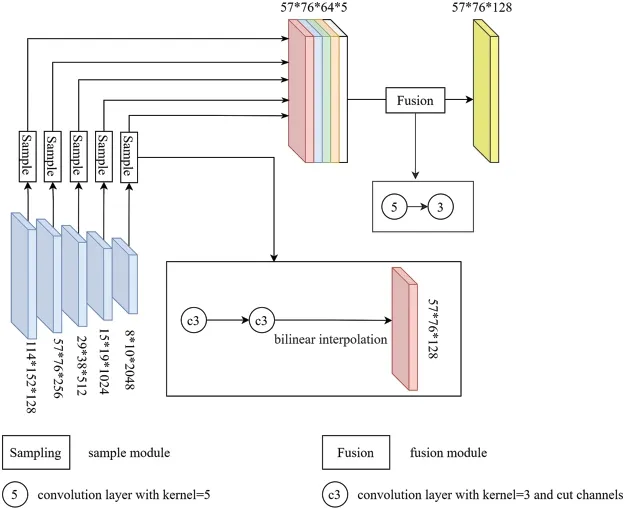
Figure 4: The architecture of the Scene Understanding module. The sample module uses to sample each scale feature to the same scale and the fusion module is used to adaptive fuse multi-scale features for learning the whole scene feature

Figure 5:The architecture of the Scale Transform module
3.3 Boundary Aware Depth Loss(BAD)
In this section, we propose a novel depth loss function Boundary Aware Depth loss (BAD) to pay attention to the loss,caused by the boundary,which is usually ignored in training.Generally,the depth value at the plane is continuous with a smoother gradient,while the depth at the boundary is discontinuous with a large gradient.The boundary area always occupies a little proportion through the gradient of the boundary is larger,which causes little loss in training.So,it is easily ignored,especially in indoor scenes,there are more planes than other scenes,due to the existence of walls,ceilings,tables,beds, etc. Therefore, the models tend to predict the depth of the entire scene with the same smooth depth when training the depth estimation model,which aggravates the boundary blur problem.To deal with the ignored loss caused by the boundary,Hu et al.[15]proposed the gradients of depth term in the total loss function to guide the model to predict the depth maps with accurate boundary gradients.However,the gradient loss term will not play an ideal role when the background and boundary,depth predicted by the model,is too large or too small at the same time.In this paper,based on Hu et al.[15],we propose a novel depth loss function BAD to pay attention to the boundary depth for improving the depth accuracy of the object boundary. BAD guides the training process by setting a boundary aware Weight for each pixel.The BAD is defined as:

LBADcontains two items, the boundary aware weight and depth predict item. Where thewboundary aware weight,dis the true depth,is predicted depths. Theαis an aware factor, we setα= 0.3 in this paper. These pixels will be focused if the boundary aware weight is big. Boundary aware weightwis defined as:
where thegxis the gradient ofxscale and thegyis the gradient ofyscale in the ground truth. Theis the gradient ofxscale and theis the gradient ofyscale in predicted depth maps. TheNis the total number of pixels. We use the Sobel operator [31] to extract the gradient in this paper. Thewincludes the true and error items,wwill enforce the model to focus on boundary area by setting different weights to these pixels.The true item will become big when these pixels have a big gradient in the ground truth. The error items will show their role if there is a large gradient prediction error.When the background and boundary depth are too large or too small at the same time,our true items and the depth error item in(1)will become big,which guides the model to focus these pixels together even though the gradient error is small.The error item is used to guide the model to focus on these boundary fields where the gradient error is big. The depth loss will be huge when the true item and the error item are big at the same time.To ensure our model can take a bigger awareness of the object boundary and point cloud quality,we retain the edge loss item and normal loss item proposed by[15].The total loss is defined as:

Extensive experiments show that BAD can improve the accuracy of the boundary and depth.
4 Experiments
In this section, we will introduce the evaluation indicators in our experiment firstly. Then we introduce the datasets used in our experiment, and finally, we conduct various experiments on the datasets to prove the effectiveness of the novel modules and functions.
4.1 Quantitative Evaluation Indexes
This paper follows [3] using the metrics to evaluate our proposed model’s performance. These metrics define as:
Root mean squared error(RMSE):

Absolute relative difference(AbsRel):

log10:

Threshold(δ)

wherethr= 1.25,1.252,1.253thegiis the ground truth,is the predict depth value, andTis the available pixels in the ground truth.
4.2 Datasets and Experimental Setting
This paper focuses on indoor scenes which have a complex scene structure with a large number of objects. So we mainly trained and evaluated our model in NYU-Depth V2 [19]. The NYU-Depth V2 [19] dataset is the most popular indoor dataset in monocular depth estimation and semantic segmentation.It uses a Kinect depth camera[32]to capture images,mainly for scene understanding.It contains 1449 pairs of RBGD image pairs with a resolution of 640*480 from 464 different indoor scenes from 3 cities. These image pairs are divided into two parts. 795 image pairs captured in 249 scenes are used as the training set, and 654 image pairs from 215 scenes are used as the test set. In addition, the data set also contains the corresponding semantic segmentation label information. In our experiment,we use the training dataset that contains 50K RGB-D images that were preprocessed by Hu et al.[15].
In this paper, we use the Pytorch [33] to implement our model, and then in the encoder state,we use the SENet-154[30]as our backbone to initialize the pre-trained model by ImageNet[34].We set the LR = 0.0001 and use the learning Adam optimizer. Furthermore, we set a rate decay policy to the learning rate by reducing it to 10% every 5 epochs, we setβ1 = 0.9,β2 = 0.999, epochs =10, and weight decay as 10-5. Our model was trained and evaluated on a two-piece Tesla V 100(32 GB version)with a patch size is 16.
4.3 Performance Comparisons
In this section, we evaluate our model from both qualitative and quantitative points of view on the NYU-Depth V2 dataset [19]. Firstly, we compare the different state-of-the-art models with our model tested on the NYU-Depth V2 dataset[19]by the common indicators and the results are shown in Table 2.From Table 2 we can see that our model shows state-of-the-art inδ2andδ3.Additionally,we also get the second state inδ1Rel. Although our accuracy is next, Reynolds et al. [16] built an FFP to get a fusion of features in each scale to improve the predicting accuracy, which leads to the model becoming big.In contrast,we only fuse features once and use the ST to transform the fusion feature to different scales.Furthermore,the output of SU only has 128 channels,which also reduces the parameters.Moreover,our main purpose of this paper is not to improve the accuracy of depth but to get clear boundaries in the depth maps.To prove our contribution to predicting clearer boundaries,we provide the qualitative results of our model, which is shown in Fig.6, which includes five group results.From Fig.6,we can see our model predicts the clearer structure than other models,even better than the ground truth, like the black boxes in the first group. The ground truth is captured by the Kinect[32]using an infrared ray,but the glass will reflect the ray which leads to depth loss in the glass.But the monocular depth estimation can predict the depth of glass.
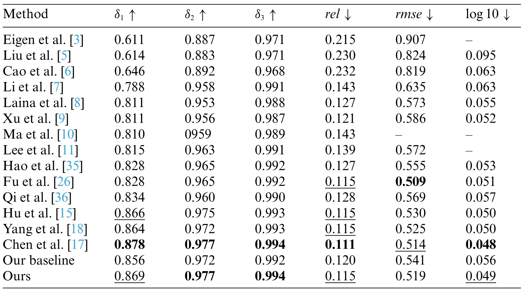
Table 2: Evaluation results of depth estimation on the NYU-Depth V2 test set. The best results are boldfaced,and the second-best ones are underlined.The shown values of the evaluated methods are those reported by the authors in their paper
In the second group,our model predicts the clearest structure of the bed with a sharp boundary.Although Chen et al.[17]and Hu et al.[15]keep the whole structure of the bed,they suffer from serious boundary smoothness leading to some structures being indistinguishable from the background.The same situation also appeared in the third group.In the third group,Chen et al.[17]and Hu et al.[15]cannot predict the toy with a clear boundary that causes the toy and the sofa to be mixed,and the toy is completely invisible from the depth map.By contrast,our model predicts the toy with an obvious boundary, the toy, and the sofa can be distinguished. In the fourth group, we can see that other methods predict fuzzy table boundaries, especially in the area selected by the black box. Although Chen et al.[17]and Hu et al.[15]also predicted the overall structure of the chair,the predicted edges of the backrest were very blurry and there was a serious smoothing phenomenon. Additionally, in the black box on the wall,we can see a chair placed on the wall from the ground truth.Our method not only successfully predicts chairs with sharp edges, but also suppresses the boundary smoothing phenomenon,so the chair and the wall are distinguished.But other algorithms did not deal with the boundary smoothing phenomenon, resulting in the wall and the chair being indistinguishable. The same situation also occurs in the fifth group,in which the other algorithms did not predict the clear boundaries between the cabinet and the table.Because the cabinet is back against the wall,the predicted depth of the display is very close to the depth of the wall.As a comparison,our model not only predicts clear boundaries but also is more discriminatory than others in the depth prediction of the display.In general,our algorithm can preserve the overall structure of the scene better than other algorithms,and can effectively distinguish objects and background thanks to our depth maps with clear boundaries.In addition,the clear boundary information also helps us to get more accurate depth predictions when the background and object depths are similar.To prove that our method estimates more accurate the depth in the edge, we evaluate the accuracy of depth in the edge region and compare it with others.The result is shown in Table 3(edge thredhold=0.5,boundary gradient threshold that was proposed in Hu et al.[15].We will regard the pixel as the boundary if its gradient is bigger than the threshold).Ours shows the best performance inδ2,δ3.

Figure 6: Qualitative results on the NYU-Depth V2 test set. From left to right: input RGB images,ground-truth depth maps,results of Eigen et al.[3],Laina et al.[8],Hu et al.[15],Chen et al.[17],and our method,respectively
4.4 Models Test in Other Dataset
To evaluate our model more thoroughly,we test our pre-trained model in the SUN RGB-D[20]directly.SUN RGB-D[20]is a scene understanding benchmark,which includes three datasets NYUDepth V2 [19], B3DO [37], SUN3D [38]. To ensure the effectiveness of the comparison, we choose Hu et al.[15],Chen et al.[17],and Yang et al.[18]as the comparison models.We use the same dataset[19]to train the model.The comparison results are shown in Fig.7.We select five sets of depth maps predicted from different scenes as a comparison.In the first group,we can see the comparison models have s.In the second group,from the black boxes,we can see that our model predicts a desktop with a clear preserved object structure of the scene,and our model’s object boundaries are the clearest(tables and chairs in the black box). The lack of depth in ground truth is due to specular reflections of the scene,which is difficult to obtain the depth in the corresponding area.This is the disable in RGB-D camera and LIDAR.This phenomenon also can be found in the second and third group boundary.What’s more, we also predict the outline of the faucet but the other algorithms do not get a clear outline, and they are very hard to distinguish the faucet from the background. In the third group,we can also see that a clearer object structure is preserved by ours than in others. From the fourth group, we can see that our model shows an obvious advantage over other algorithms in structural preservation,it retains the complete object structure while also getting sharp boundaries.This makes the object can be perfectly distinguished from the background. In other algorithms, it is sometimes difficult to distinguish the object from the background due to the blurry structure and smooth edges.Moreover,the object is easily mistaken as the background when the edges are blurry.

Table 3:Evaluation results of edge depth estimation on the NYU-Depth V2 test set.The best results are boldfaced,and the second-best ones are underlined
As can be seen in the last group,our model predicts sharper table legs compared to other models.This experiment is used to prove that our model can predict the depth map with a clear boundary.
Furthermore, it will have a depth value similar to the background, resulting in huge errors. To explore the performance of our model, we test our pre-trained model on iBims-1 dataset [21] and compare it with others. The result is shown in Table 4. We can see that our model shows the stateof-art inδ1,δ2,δ3,rel, and log 10. The result shows that the model proposed in this paper has great generalization.
We show the visual result in Fig.8 which includes four comparison groups.In the first group,we can see that our methods save the clearest outline of the lamp than others.Ours maintain the structure of windows that others without in the second group.In the third group,ours saves more detail in the plant and the boundaries are clearer than other methods. In the last group, our predicted saves the structure of windows and shelves that others cannot keep. As mentioned above, our methods show excellent performance in saving the detail of the object and predicting clearer boundaries.
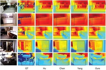
Figure 7: Qualitative results of the test on the SUN RGB-D. From left to right: input RGB images,ground-truth depth maps, results of Hu et al. [15], Chen et al. [17], Yang et al. [18], and our method,respectively
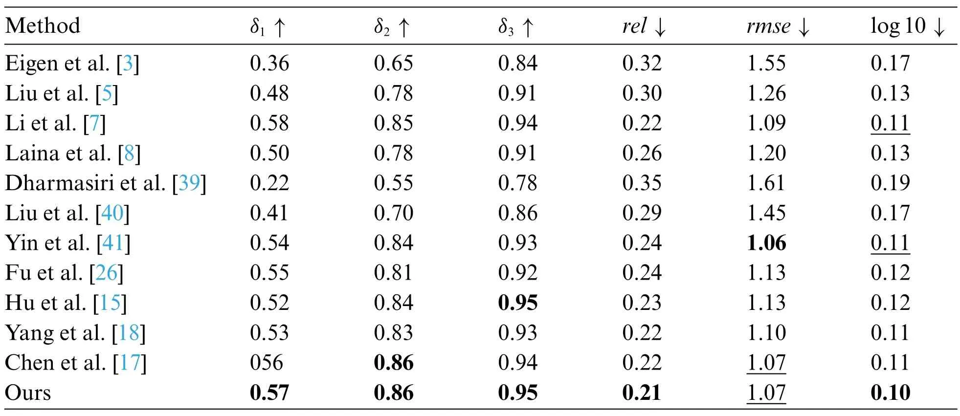
Table 4: Evaluation results of depth estimation on the iBims-1 dataset [21]. The best results are boldfaced,and the second-best ones are underlined

Figure 8:Qualitative results of the test on the iBims-1 dataset.From left to right:input RGB images,ground-truth depth maps,results of Hu et al.[15],Chen et al.[17],Yang et al.[18],and our method,respectively
4.5 Boundary Accuracy Comparisons
To prove that our model can predict more accurate boundaries than others more effectively, we compare them to specific evaluation indicators.We follow Hu et al.[15]using the Precision,Recall,and F1 scores to evaluate the method performance,the results show in Table 5.There is the boundary gradient threshold that was proposed in Hu et al.[15].We will regard the pixel as the boundary if its gradient is bigger than the threshold.We can see that our model has achieved 3 SOTA and 5 sub-SOTA in 3 indicators with 3 different thresholds.The results prove that our model performs SOTA in edge accuracy.
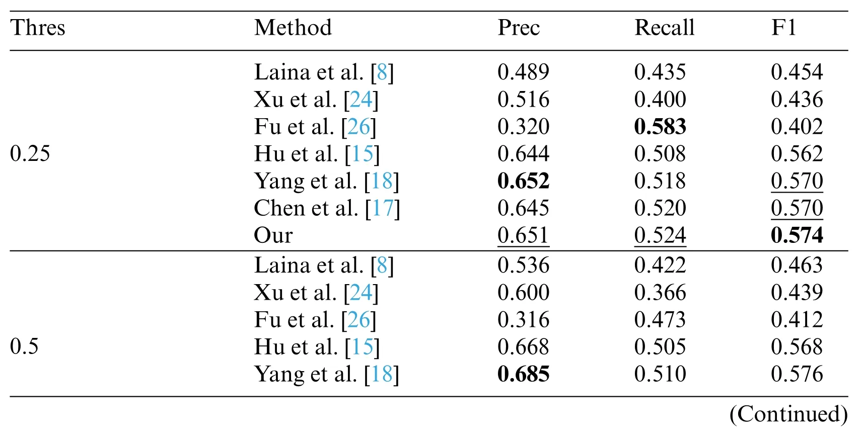
Table 5: Accuracy of recovered edge pixels in-depth maps under different thresholds based on NYU-D V2 test set.The best results are boldfaced,and the second-best ones are underlined(Thres is the boundary gradient threshold that was proposed in Hu et al.[15])
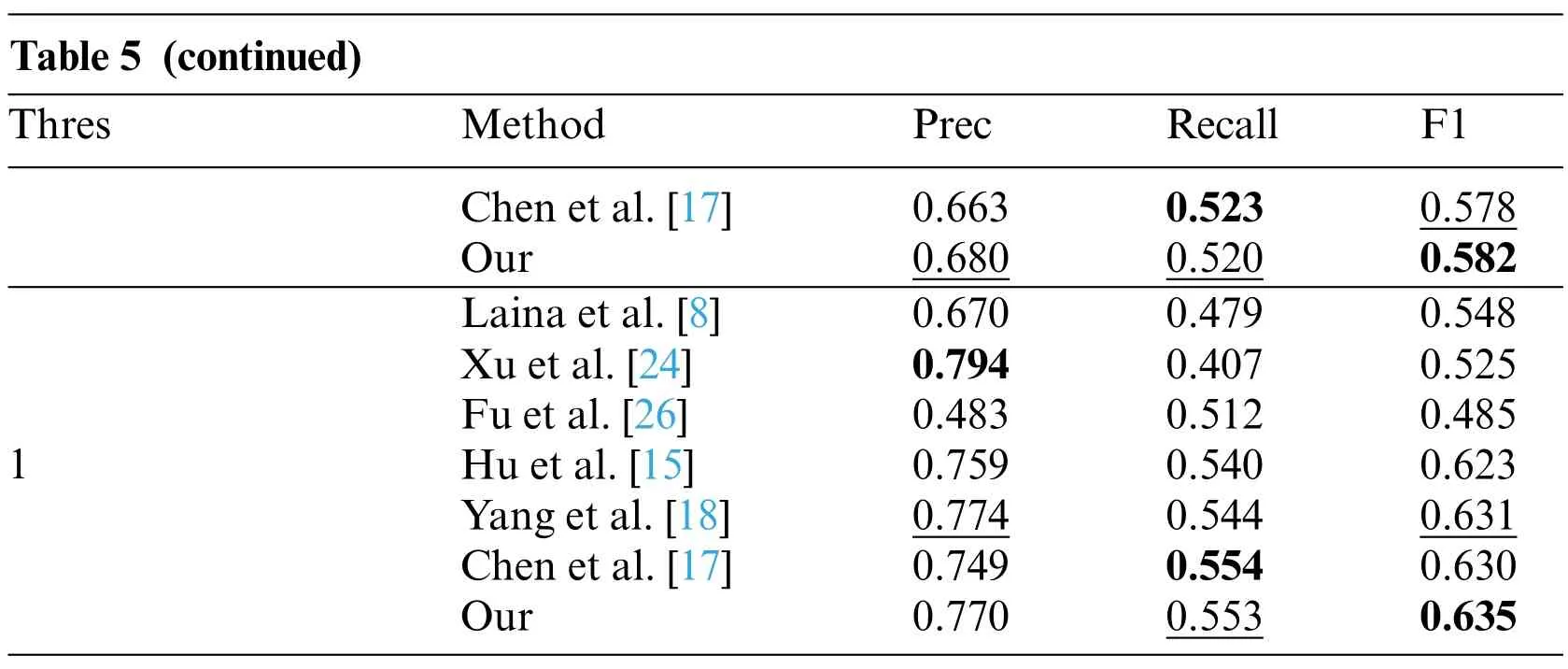
Table 5 (continued)Thres Method Prec Recall F1 Chen et al.[17] 0.663 0.523 0.578 Our 0.680 0.520 0.582 1 Laina et al.[8] 0.670 0.479 0.548 Xu et al.[24] 0.794 0.407 0.525 Fu et al.[26] 0.483 0.512 0.485 Hu et al.[15] 0.759 0.540 0.623 Yang et al.[18] 0.774 0.544 0.631 Chen et al.[17] 0.749 0.554 0.630 Our 0.770 0.553 0.635
4.6 Generating Point Cloud from Depth Maps
As mentioned in the pre-chapters,the sharp boundary can suppress“flying pixels”effectively in the point clouds projected by depth maps.To prove this conclusion,we projected the predicted depth maps as 3D point clouds and rendered them in novel views using OpenCV.The results are presented in Fig.9.From the first group,other algorithms have serious pixel drift in the head of the man in the red block.Our algorithm suppresses this phenomenon well and the point cloud in the head of man is continued.The same situation also appeared in the second set.The projection effect of Hu et al.[15]is relatively good,but it still appears seriously distortions at the upper boundary of the screen.Compared with others,our model also has distortions at the bottom edge of the screen,but the overall structure is better than others.In the third group,we can see that all methods have better preserved the overall structure of the scene.However,by changing the perspective,we found that the TV screen predicted by other methods has serious“flying pixels”and the screen is distorted which surface is curving.Although ours suffers a slight of flying pixels at the top of the screen,the overall screen is not distorted.Through point clouds comparison experiments,we proved that our algorithm can suppress the phenomenon of“flying pixels”effectively, and also proved the opinion that accurate edge information can help to improve the quality of the point clouds project from depth maps.
4.7 The Comparison of Model’s Params
To prove that the ST can show a great performance in reducing the number of params,we make the comparison between ours and others and the comparison results can be seen in Fig.10. From Fig.10,we find that our model’s parameters are slightly more than Hu et al.[15].That is because[15]just fused the multi-scale feature one time on a single scale and did not change the fusion feature to different scales. But our model not only fuses the all-scale feature in every training process but also transforms the fusion feature into 5 different scales.What’s more,Compared with Chen et al.[17]and Yang et al.[18]who built the FFP,our model only contains two-thirds of the parameters of these FFP models.
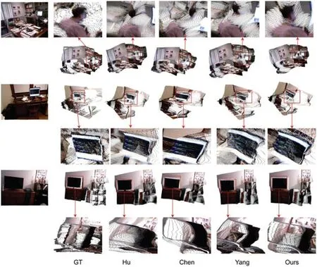
Figure 9: The result of comparing the projected point cloud from ours and other methods. From left to right: input RGB images, ground-truth depth maps, results of Hu et al. [15], Chen et al. [17],Yang et al.[18],and our method,respectively
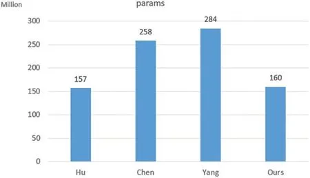
Figure 10: Compare the number of model’s params. From left to right: results of Hu et al. [15],Chen et al.[17],Yang et al.[18],and our method,respectively
4.8 Ablation Studies
To explore our model in detail,we designed corresponding ablation experiments for the proposed method.The results are shown in Tables 6 and 7 based on thresholds=0.5.The first group experiment is mainly to show the performance of the baseline as the benchmark for subsequent comparisons.For the baseline, we use SeNet154 [30] as the backbone and use the composite loss function proposed by Hu et al. [15] to supervise the model training. From the results of the second group, it can be known that directly adding BAD to supervision model training can improve the prediction accuracy of the model effectively. Comparing the third group and the baseline, we can see that the SU+ST can show a great enhancement in the model performance.To confirm the effectiveness of ST,we use bilinear interpolation to sample the output of the SU to different scales directly in the fourth group.Comparing the fourth group with the fifth group we can find that the fifth group which uses the ST shows more accurate performance than the fourth group which uses bilinear interpolation directly.The comparison between the second group and the fourth group proves that SU can effectively improve the functioning of the model.In particular,there is a major improvement in edge accuracy.Comparing the third group with the fifth group we can see that the BAD shows a great promotion of the model’s performance.

Table 6:The depth accuracy comparison.With our module or without.The best results are boldfaced,and the second-best ones are underlined

Table 7:The edge accuracy comparison,with our module or without.The best results are boldfaced,and the second-best ones are underlined
5 Conclusion
To deal with the blurry boundary caused by low-level information loss in the process of feature extraction and boundary smoothness in the boundary area during the training process, a Scene Understanding module,a Scale Transform module,and a Boundary Aware Depth loss function were proposed.In the Scene understanding module and Scale Transform module,we focus on taking care of information loss. The Scene understanding module can learn the global information about the scene and the Scale Transform module will transform the global scene information to multi-scale for building a feature pyramid with a few additional parameters. The Boundary Aware Depth loss was designed to enforce the model to focus on the depth in the boundary field during the model training.Extensive experiments show our modules and the novel loss functions ensure our model can predict depth maps with clearer object boundaries than others.The most important thing is the object will be predicted with the depth value the same as the background without a clear boundary.It means that the boundary information can influence the depth prediction.But some problems still exist,for example,although our model can recover the boundary very well,the point clouds are not always nice enough.Such as some plants are not smooth.The other problem is the complex time of our model is high.In future work,we will concentrate on how to improve the accuracy of depth prediction and reduce the time complexity.Also,we will further explore the influence of object boundaries in depth prediction.
Funding Statement:This work was supported in part by School Research Projects of Wuyi University(No.5041700175).
Conflicts of Interest:The authors declare that they have no conflicts of interest to report regarding the present study.
 Computer Modeling In Engineering&Sciences2023年7期
- Computer Modeling In Engineering&Sciences的其它文章
- Edge Intelligence with Distributed Processing of DNNs:A Survey
- Turbulent Kinetic Energy of Flow during Inhale and Exhale to Characterize the Severity of Obstructive Sleep Apnea Patient
- The Effects of the Particle Size Ratio on the Behaviors of Binary Granular Materials
- A Novel Light Weight CNN Framework Integrated with Marine Predator Optimization for the Assessment of Tear Film-Lipid Layer Patterns
- Implementation of Rapid Code Transformation Process Using Deep Learning Approaches
- A New Hybrid Hierarchical Parallel Algorithm to Enhance the Performance of Large-Scale Structural Analysis Based on Heterogeneous Multicore Clusters
