SYMBOLIC COMPUTATION FOR THE QUALITATIVE THEORY OF DIFFERENTIAL EQUATIONS∗

Bo HUANG()

LMIB–School of Mathematical Sciences,Beihang University,Beijing 100191,China

E-mail:bohuang0407@buaa.edu.cn

Wei NIU()†

Ecole Centrale de Pekin,Beihang University,Beijing 100191,China;Beihang Hangzhou Innovation Institute Yuhang,Hangzhou 310051,China

E-mail:Wei.Niu@buaa.edu.cn

Dongming WANG()

LMIB–Institute of Artifi cial Intelligence,Beihang University,Beijing 100191,China;Centre National de la Recherche Scientifi que,75794 Paris Cedex 16,France

E-mail:Dongming.Wang@lip6.fr

Abstract This paper provides a survey on symbolic computational approaches for the analysis of qualitative behaviors of systems of ordinary differential equations,focusing on symbolic and algebraic analysis for the local stability and bifurcation of limit cycles in the neighborhoods of equilibria and periodic orbits of the systems,with a highlight on applications to computational biology.

Key words biological systems;center-focus;limit cycles;qualitative analysis;symbolic computation

Dedicated to Professor Banghe LI on the occasion of his 80th birthday

1 Introduction

Since the pioneering work of Poincar´e [1]and Liapunov [2],the qualitative theory of differential equations has been developed and used as a powerful tool for analyzing the qualitative behaviors of dynamical systems of differential equations without solving the systems.The theory has played an indispensable role in the study of differential equations,as few such equations can be solved explicitly.The theory has also become a fundamental part of graduate and undergraduate curricula in analysis,taught in most departments of mathematics as a standalone course(see,e.g.,the popular textbooks by Nemytskii and Stepanov [3],Zhang and others [4]).

The analysis of qualitative behaviors of dynamical systems involves heavy computations with large symbolic expressions which can neither be performed numerically using limited precision,nor be done effectively by hand for the complexity in question.Fortunately,advanced software tools,implemented along with newly developed algebraic methods on modern computers,have become available for efficient symbolic computation,helping make the qualitative theory of differential equations practically more powerful.Notably,in 1985,Qin and others [5]initiated computer-aided derivation of stability criteria for certain cubic differential systems.In 1988,Wang [6]implemented a mechanical procedure to compute Liapunov constants for polynomial differential systems of center-focus type.By using that procedure and the methods of characteristic sets [7]and Gröbner bases [8],Jin and Wang [9]rediscovered the incompleteness of Kukles’center conditions of 1944.Since then,the so-called Kukles problem has stimulated a lot of research interest in center conditions and the bifurcation of limit cycles,see [10–14]for instance.In the past few decades,symbolic methods have been explored extensively in terms of the qualitative analysis of dynamical systems.The problem of tedious deductions involved in the analysis has been resolved to a large extent,and many encouraging results have been obtained regarding the stability analysis of dynamical systems [15–17],the determination of center conditions [6,18,19],the estimation of the number of limit cycles [20–22],etc.

This article reviews the recent progress on symbolic and algebraic computation methods for the qualitative theory of differential equations.The paper is organized as follows:several well-known algebraic methods are recalled briefly in Section 2,and then used in Section 3 to deal with the algebraic problems formulated from stability analysis.In Section 4,we show how bifurcation analysis may be carried out by using algebraic methods as well.In Section 5,Poincar´e’s method for computing Liapunov constants and a brief account of the research on using symbolic approaches to the center-focus problem are presented.Sections 6 and 7 are devoted to the study of the bifurcation of limit cycles.We highlight results obtained from two types of bifurcations:one is the well-known Hopf bifurcation of limit cycles and the other is the bifurcation of limit cycles from the periodic orbits of period annuli.Two important and widely used methods(the Melnikov function method and the averaging method)for studying thenumber of limit cycles of nonlinear differential systems are also discussed.Section 8 presents the application of algebraic methods to the qualitative analysis of biological systems.The paper is concluded with a few remarks.

2 Symbolic Computation and Detection of Equilibria

Symbolic computation is a scientific area that refers to the study and development of algorithms and software tools for manipulating mathematical expressions and objects.Polynomial system solving is a fundamental problem in symbolic computation;its main objective is to study the structures and representations of solutions for systems of polynomial equations(=),inequations()and inequalities(>)and to develop efficient methods and software tools for the computation of such representations.Symbolic methods for solving polynomial systems can be divided into two categories:one dealing with systems of polynomial equations and inequations over any field by means of variable elimination and triangular decomposition,and the other dealing with systems of polynomial equations and inequalities over the field R of real numbers using real quantifier elimination and real polynomial system solving.

2.1 Solving Systems of Algebraic Equations

Most of the methods for solving systems of polynomial equations and inequations symbolically are based on the theories of Gröbner bases,triangular sets,and resultants.The notion of Gröbner bases was introduced originally by Buchberger in his Ph.D.thesis [23].Gröbner bases of polynomial ideals are specially structured sets of generators of the ideals.They can be computed from any given sets of generators of the ideals and have many nice properties.Gröbner bases can be used to solve plenty of problems concerning polynomial ideals,such as primary ideal decomposition,ideal membership test,and polynomial system solving.The method has been well studied in the area of symbolic computation with important theoretical and practical improvements made by many prominent researchers.Successful use of techniques of linear algebra for fast polynomial reductions led to highly efficient algorithms such as FGLM [24,25],F4[26]andF5[27]for the computation of zero-dimensional Gröbner bases.

Triangular sets are special sets of multivariate polynomials which may be ordered in a certain triangular form.They have nice structures and are suitable for representing field extensions and zeros of polynomial systems of any dimension.There are various kinds of zero decompositions that may be applied naturally to solving systems of polynomial equations and inequations.Characteristic sets are special triangular sets.The method of characteristic sets,developed by Wu [7,28]on the basis of the classical work of Ritt [29],and so named after Wu and Ritt,is another fundamental method of algorithmic polynomial algebra.Wu–Ritt’s method and the theory of triangular sets and systems have been studied,improved,and extended by many researchers(see,e.g.,[30,31]and references therein).

Resultants provide a simple and effective way to eliminate one or several variables simultaneously from a given set P of polynomials,allowing one to triangularize P or to establish conditions for P to have zeros;see [31,Section 5.4]and [32,Section 3],and references therein,for more information about the classical theory and modern developments on resultants.

2.2 Solving Semi-Algebraic Systems

Systems involving equations and inequalitiesover Rarecalled semi-algebraic systems.Most of the methods for solving semi-algebraic systems are based on cylindrical algebraic decomposition(CAD),real solution classification(RSC)and discriminant varieties(DV).

CADThe CAD method,invented by Collins [33],is fundamental for computer algebra and real algebraic geometry.The basic idea underlying the method is to decompose Rninto finitely many cylindrically arranged regions,called cells,such that the input polynomials all have constant signs over each cell.The cells are all semi-algebraic,so that they can be described by semi-algebraic systems.The invariance of signs makes it easy to determine the signs of all of the polynomials in each cell by computing the values of the polynomials at a sample point in the cell,thus allowing one to eliminate the quantifiers of any quantified formula and for classifi cation of real solutions of semi-algebraic systems.Collins’algorithm consists of two key phases:projection and lifting.In the projection phase,one projectsn-variate polynomials to(n−1)-variateonesby eliminating onevariableusing an appropriateprojection operator,then to(n−2)-variateones,and finally to univariatepolynomials.There have been numerous extensions and improvements over Collins’original CAD algorithm.One of the notable improvements was made by Collins and Hong [34]for the lifting phase by constructing a partial CAD.

RSCYang and Xia [35,36]proposed a practical method for thereal solution classifi cation of an arbitrary semi-algebraic system S.The method works by computing a border polynomialBin the parameters µ =(µ1,···, µd),which is a product of polynomialsqi( µ )such thatBsatisfies two conditions:the number of distinct real solutions of S is invariant in each connected component of the complement ofB=0 in Rd,and if all of the signs ofqiare the same in two components,then the number of distinct real solutions of S remains the same in these two components.After the polynomialBis obtained,one can obtain sample points in each connected component of the complement ofB=0 and then isolate the distinct real solutions of S at each sample point.Finally,the signs of the factors ofB,together with the numbers of real solutions of S at the sample points,can be obtained,and the necessary and sufficient conditions for S to have a prescribed number of distinct real solutions can be expressed by the signs of the factors ofB.

DVThe discriminant variety of a semi-algebraic system

wasdefined by Lazard and Rouillier in [37].Here µ =(µ1,···, µd)is the sequence of parameters and x=(x1,···,xn)is the sequence of variables in the system.A discriminant varietyVof a semi-algebraic system of the form(2.1)is a semi-algebraic subset of the real space Rdof the parameters µ satisfying the property:on each connected open subset of Rdnot meetingV,the number of real distinct solutions of the polynomial equationsformed by thepi’sis constant and the signs of all theqj’s at these real solutions are invariant.

While speaking about the methods of symbolic computation in this paper,we mean,nonexclusively,the algebraic methods of resultants,Gröbner bases,characteristic sets,triangular decomposition,CAD,quantifier elimination(QE),RSC,and DV,as mentioned above,which can be used to solve algebraic and semi-algebraic systems of polynomial equations,inequations,and inequalities,and to study the properties and relations of algebraic and geometric objects defined by the real or complex solutions of such systems.There are a number of advanced software packages available for computing Gröbner bases,triangular sets and zero decompositions,resultants,and discriminant varieties,and for doing real solving,solution classifi cation,and quantifier elimination.The reader may consult [38]for more information about such software packages.

2.3 Detection of Equilibria

Consider autonomous systems of ordinary differential equations of the form

whereP1,···,PnandQ10,···,Qn0 are polynomials in µ =(µ1,···, µd)and x=(x1,···,xn)with rational coefficients, Ω is the set of polynomial equations,inequations,and inequalities in µ and x with rational coefficients,and µ are real parameters independent oft.

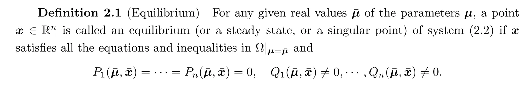
Therefore,the general problem of determining the(number of)equilibria of(2.2)can be reduced to that of finding the(number of)real solutions of the following semi-algebraic system:

This algebraic problem can be solved by using the algebraic methods mentioned above.

3 Symbolic Analysis of Local Stability

We recall the method of Liapunov with the technique of linearization to analyze the local stability of equilibria of system(2.2).

3.1 Liapunov’s First Method

Consider then×nJacobian matrix of system(2.2),

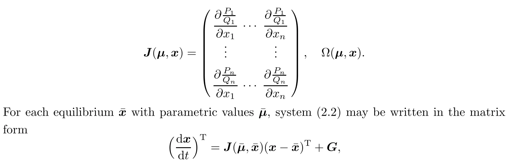
where the superscript T denotes a matrix transpose,and

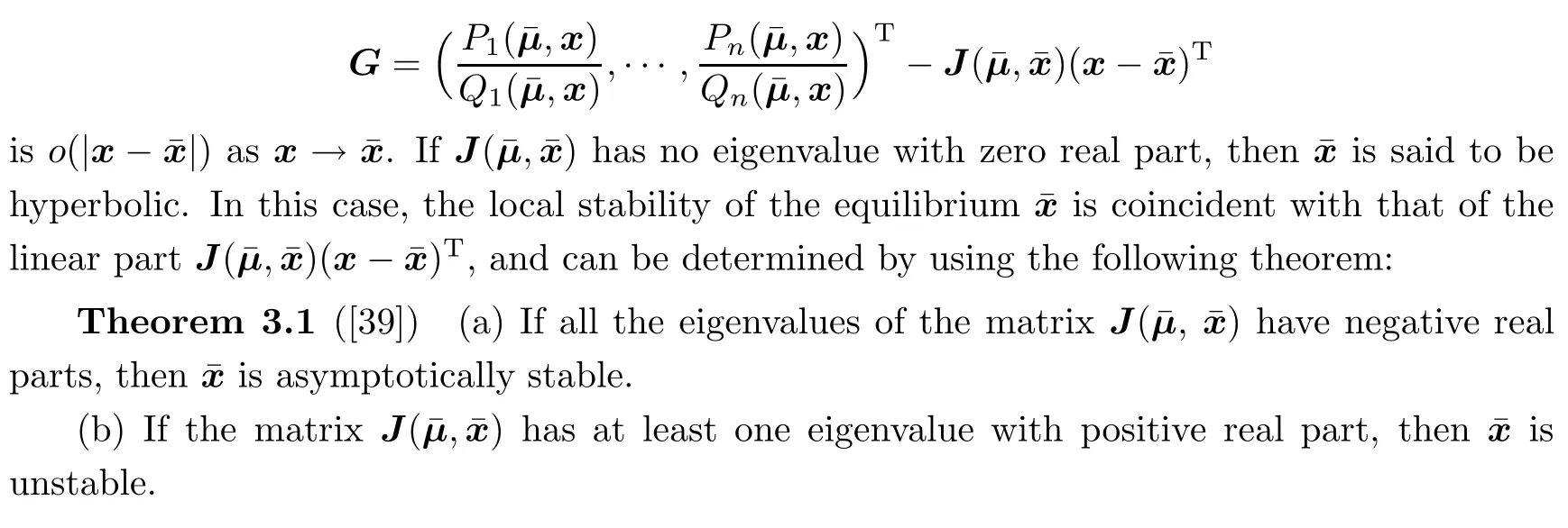
3.2 Criteria for Local Stability Analysis

For any high-dimensional differential system of the form(2.2)withn>2,the two criteria listed below may be used to determine whether all the eigenvalues of the Jacobian matrixhave negative real parts.A univariate polynomialAwith real coefficients is said to be stable if the real parts of all the roots ofAare negative.In particular,

may take the characteristic polynomial of

Routh–Hurwitz CriterionLetAbe a real polynomial inλas in(3.1),and assume thatan>0(ifan<0,thenAmay be scaled by−1,which does not change the zeros ofA).

Defi ne then×nmatrix

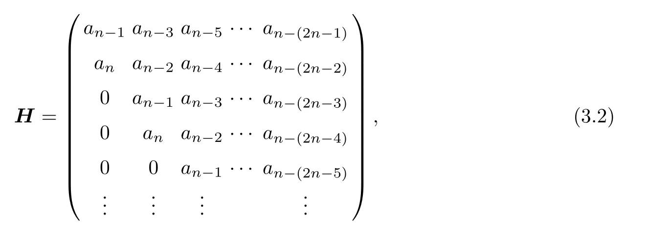
whereai=0 fori<0.H is called the Hurwitz matrix associated withA.Let∆1,∆2,···,∆nbe the leading principal minors of H,known as the Hurwitz determinants ofA.

Theorem 3.2(Routh–Hurwitz Criterion [39])The polynomialAis stable if and only if

Expanding∆nalong the last column,one can easily see that∆n=a0∆n−1.Therefore,condition(3.3)is equivalent to

Li´enard–Chipart CriterionLi´enard and Chipart [40]showed that only about half of the Hurwitz determinants are indeed needed,and the remaining Hurwitz determinants may be replaced by certain coefficientsaiofA.

Theorem 3.3(Li´enard–Chipart Criterion [40])The polynomialAis stable if and only if one of the following four conditions holds:

Heremandm′are the integer parts ofn/2 and(n+1)/2,respectively,and∆1,∆2,···,∆nare the Hurwitz determinants ofA.

3.3 Stability Analysis by Solving Semi-Algebraic Systems

LetH1,···,Hrbe polynomials in µ and x with rational coefficients.In practice,Himay take some of theaiand∆jmentioned above.For the problem of local stability analysis,Wang and Xia [16]formulated it as an algebraic problem and proposed a general method to solve the problem via symbolic computation.The method,extended later by Niu and Wang [41],applies to any differential system of the form(2.2),though its target application was for biological systems.

The algebraic problem of stability analysis can be further reduced to the problem of solving the semi-algebraic system

whereΥis a set of inequalities involvingH1,···,Hr.For example,if one needs to determine the conditions for system(2.2)to have a given number of stable equilibria,then Υ should be {H1>0,···,Hr>0}.

The method of quantifier elimination has also been applied to the problem of stability analysis.Hong and others [15]showed that the stability analysis for continuum and discrete initial boundary-value problems can be stated in terms of QE problems and then be solved by using the method of partial CAD.Moreover,Jirstrand [42]applied the method of partial CAD to nonlinear control system design.However,Liapunov’s first method of linearization does not work at the bifurcation points where the Jacobian matrix has eigenvalues with zero real parts.In this case,local stability is usually analyzed by checking the existence of a local Liapunov function.She and others proposed methods for automatically discovering local Liapunov functions in quadratic forms [43]and beyond quadratic forms [44],based on the method of real solution classification.

4 Symbolic Analysis of Bifurcations

Stability analysis based on the technique of linearization presented in Section 3 fails at bifurcation points becausenear such points thebehavior of system(2.2)may differ qualitatively from that of its linearized system,and bifurcation may occur(see,e.g.,[4,39,54]).Even for autonomous systems there may be many different bifurcating situations whose study is a highly nontrivial task and requires sophisticated mathematical methods and effective computational tools.

4.1 Planar Differential Systems

We start with planar polynomial differential systems,i.e.,systems of the form(2.2)withn=2 andQ1=Q2=1,which can be written as follows:

Hop f BifurcationThere are different situations in which bifurcations at an equilibrium of the dynamical system(4.1)may occur.In one of the most important situations,the Jacobian matrix J( µ ,x)of(4.1)at the equilibrium has a pair of purely imaginary eigenvalues but no other eigenvaluewith zero real part.Thebifurcation in thissituation iscalled a Hopf bifurcation or an Andronov–Hopf bifurcation(see [133],for example).Hopf bifurcation leads to the birth of limit cycles from equilibria of dynamical systems,when the equilibria change their stability via the movements of the imaginary eigenvalues away from the imaginary axis.

Let the characteristic polynomial of J( µ ,x)beλ2+pλ+q.Then Hopf bifurcation may occur whenp=0 andq>0.To determine conditions on µ for the existence of Hopf bifurcation points,one may consider the quantified formula

where the logical conjunctionP∧Qis equivalent toPandQ.From the above formula,the conditions may be obtained as a quantifi er-free formula by eliminating the quantifi ers.More discussions of Hopf bifurcation can be found in Section 6.

Saddle-Node BifurcationWhen J( µ ,x)has one zero eigenvalueand one negative real eigenvalue,i.e.,p>0 andq=0,saddle-node bifurcation occurs.This bifurcation may be of several kinds,according to the different changes of equilibria and stable equilibria,and it occurs most often.

The problem of checking whether the equilibria of system(4.1)are saddle-node bifurcation points(when no parameter is involved),or of determining the conditions on µ (when they are present)for the equilibria to satisfy the conditionsp>0 andq=0,can be obtained by eliminating the quantifi ers from the following formula

Then one can determine the stability and types of the bifurcation points by using the classical theorem of bifurcation(see [4]for example).Based on thetheorem,Niu and Wang [45]proposed a method for analyzing saddle-node bifurcation by using symbolic computation.

Bogd anov-Takens BifurcationNow consider the case of Bogdanov–Takensbifurcation(see [4]for example),for which the Jacobian matrix J( µ ,x)hastwo zero eigenvalues,but where not all of the elements in the Jacobian matrix arezero,i.e.,p=0,q=0,but|a|+|b|+|c|+|d|0,wherea,b,c,anddare the elements of J( µ ,x).By means of quantifier elimination or by solving the algebraic or semi-algebraic system

one can decide whether an equilibrium of system(4.1)is a Bogdanov–Takens bifurcation point(when no parameter is involved)or determine the conditions on µ (when they are present)for the equilibrium of(4.1)to satisfy the conditionsp=0 andq=0.Similarly to the case of saddle-node bifurcation,the stability and types of bifurcation points may be further analyzed by using algebraic methods.

The analysis of these three bifurcations for a model of a self-assembling micelle system by using symbolic computation was performed in [45].

4.2 High-Dimensional Systems

For high-dimensional differential systems of the form(2.2),the analysis of bifurcations becomes complicated.Most studies are concerned with Hopf bifurcation,where the Jacobian matrix J( µ ,x)has a pair of complex conjugate eigenvalues and no other eigenvalue with zero real part.

Different algorithms for detection of Hopf bifurcation points based on algebraic techniques have been proposed in the literature(see [46,47,52]).For example,an efficient algorithm is described in [47]for detecting Hopf bifurcation points based on the algebraic properties of polynomial resultants and matrix-symmetric products.An implementation of the algorithm together with applications to three examples from neurophysiology can be found in [48].On the other hand,numerical methods for computing such points have also been proposed and implemented(see,e.g.,[49,50]).

Algebraic criteria for simple Hopf bifurcations were established by Liu [51]and by El Kahoui and Weber [52]independently,using different methods of proof.By simple Hopf bifurcations,we mean that the Jacobian matrix has a pair of complex conjugate eigenvalues and that all of the other eigenvalues have negative real parts.Such criteria are given in terms of the Hurwitz determinants and the constant term of the characteristic polynomial of the Jacobian matrix.

Theorem 4.1([51])LetA=anλn+an−1λn−1+···+a0withan>0 and∆1,···,∆nbe the Hurwitz determinants ofA.Then Hopf bifurcation occurs when the following conditions are satisfied:

(a)Eigenvalue conditions:a0>0,∆n−1=0,∆n−2>0,···,∆1>0.

(b)Nondegeneration condition:∂∆n−1/∂ µi/0,whereµiis one of the parameters.

To derive conditions for the occurrence of Hopf bifurcation,one may form the quantified formula

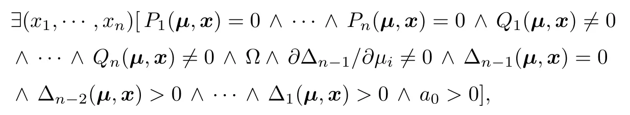
and find the conditions on µ by eliminating the quantifi ers using QE methods.

After the conditions are obtained,one can analyze the bifurcation and consider the problem of limit cycles.There are two main kinds of strategies for the bifurcation analysis of high-dimensional systems:generalizing the methods and theorems for planar systems to highdimensional ones,and reducing the problem of bifurcation analysis of systems of dimensionn>2 to those of planar systems.The former,based on the generalized Poincar´e–Bendixon theorem and the describing function method(see [53]for example),are applicable to certain types of high-dimensional systems.For the reduction of bifurcation analysis of a high-dimensional system to a planar one,the key is to keep signifi cant aspects of the dynamical characters unchanged.Using the methods of center manifold [54]and Liapunov–Schmidt reduction [55],around an equilibrium,one may be able to reduce any system of dimensionn>2 whose Jacobian matrix has no positive real part to a planar system without losing any signifi cant aspect of the dynamical characters.These methods,in combination with the approach for planar systems presented in Section 6,may be used for algebraic analysis of bifurcation and limit cycles in high-dimensional systems.

In the high-dimensional case,there may exist several kinds of bifurcations of a codimension greater than 1,and the situations of bifurcations may become more and more complex as their codimensions increase.For example,for systems of dimension 3 or higher,there may exist saddle-node Hopf bifurcation(also called fold-Hopf bifurcation),which is a local bifurcation of codimension 2,and at which the Jacobian matrix of the system at the equilibrium has a zero eigenvalue and a pair of purely imaginary eigenvalues.Another example of local bifurcation for systems of dimension 4 or higher is Hopf-Hopf bifurcation(also called double-Hopf bifurcation),at which the Jacobian matrix of thesystem at theequilibrium hastwo pairsof purely imaginary eigenvalues(see [56],for example).Such kinds of bifurcations are not simple combinations of two bifurcations.One needs to consider the actions of the two bifurcations and the interactions between them.So far there has been little work on the analysis of codimension 2 bifurcations for continuous systems using symbolic computation.

5 The Center-Focus Problem

Now we consider planar differential systems of center-focus type.In canonical coordinates,such systems are of the form

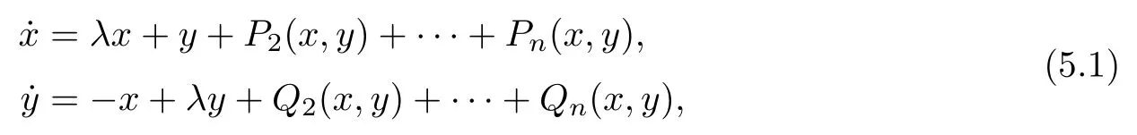
wherePiandQiare homogeneous polynomials of degreei(i=1,2,···,n).The main analytic technique to determine whether or not the origin is a center of system(5.1)was introduced by Poincar´e [1]and developed by Liapunov [57].It consists of looking for a formal power series ofxandyof the form

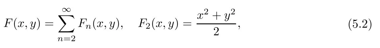
where eachFn(x,y)is a homogeneous polynomial of degreen.Let us require that dF/dtalong the orbits of(5.2)is of the form

or

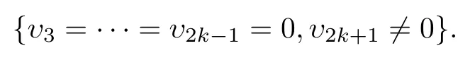
where eachV2korυ2k−1is a polynomial in the coefficients of system(5.1),which is called thekth Liapunov constant or focal value fork≥1.The origin is said to be a fine focus ifλ=0.The origin is said to be a fine focus of orderkifV2=V4=···=V2k=0 butV2k+20 orυ1=υ3=···=υ2k−1=0 butυ2k+10.Clearly,the stability of the origin is determined by the sign of the first nonvanishing Liapunov constant,and the origin is a center if and only if all the Liapunov constants are zero.

It is possible to calculate the Liapunov constants by hand only in the simplest situations.Several algorithmshavethereforebeen developed and implemented in computer algebra systems for the computation of Liapunov constants(see,e.g.,[6,18,58–60]).For polynomial systems of the form

we have uniqueness for the Liapunov constants in the sense of the following theorem,due to Shi [61]:

Let J be the ideal of A generated by all the Liapunov constants.According to Hilbert’s basis theorem,J is finitely generated,that is,there existW1,···,Wqsuch that J is generated byW1,···,Wq.Such a set of generators is called a basis for J.The vanishing of these generators implies the vanishing of all the Liapunov constants.Notice that Hilbert’s basis theorem assures us of the existence of a finite basis of generators,but it does not provide us with a constructive method to find the basis.One of the main difficulties is that the Liapunov constantVikbecomes larger and larger in terms of size askincreases,and there is no efficient algorithm to find simple sets of generators for the ideal J.The following problem has been longstanding(see,e.g.,[19,62]):

Op en ProblemFind a finite basis of generators for the ideal generated by all the Liapunov constants of a given system of the form(5.5).

A number of results on the problem of centers for polynomial systems were obtained by using the Poincar´e–Liapunov method(see e.g.,[11,63,64]).The center conditions for the quadratic system(n=2 in(5.5))were established by Dulac [65]and Bautin [66].It is well known that,for the quadratic system,the so-called Baut in ideal B is generated by the first three Liapunov constants of the system(see,e.g.,[19,66]).Moreover,the center variety V(B)⊂R6decomposes into four irreducible components,

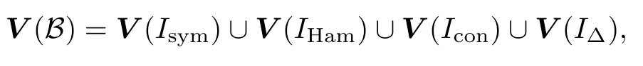
corresponding to reversible systems,Hamiltonian systems,the Zariskiclosure of systems having an invariant conic and an invariant cubic,and the Zariski closure of systems having three invariant lines,respectively.

In the cubic case with homogeneous nonlinearities,thanks to Sibirskii [67]and˙Zoladek [63],it is known that there are five independent Liapunov constants.There are many partial results for the centers of cubic systems.Unfortunately,at present,we are still very far from a complete classifi cation of all the centers of cubic polynomial differential systems.In general,it is difficult to obtain the complete classification of centers from Liapunov constants because the amount of computation required is huge(see [58]and references therein).

Let us consider a special family of cubic systems which is equivalent to a class of secondorder differential equations and can be written in the following form:

This system was first studied by Kukles [68],who claimed that the origin is a center if and only if one of the following conditions holds:

where

andξ=3a7+a2a3.The above conditions were accepted widely and included in classic textbooks(see,e.g.,[3,p.124]).In 1978,Cherkas [69]found the incompleteness of Kukles’conditions and gave a set of conditions(C1)instead of(K 1).He also proved that,fora7=0,his conditions coincide with Kukles’.Research interest in Kukles’system(5.6)was revitalized in 1988,when Jin and Wang [9]rediscovered the incompleteness of Kukles’conditions with the following example:

Christopher and Lloyd [10]immediately confirmed the computations of Jin and Wang using the computer program FINDETA.They also considered a subclass of the Kukles system,in which the coefficienta7is zero,and proved that the order of a fine focus is at most 5.Later on,other center conditions(denoted(CLP))which are not covered by Kukles’conditions were found by Christopher [12]and Lloyd and Pearson [11].

Wang [70]studied the relations among the above-mentioned conditions by applying combined elimination methods based on characteristic sets [7],Gröbner bases [8]and triangular systems [72].He proved that the center conditions(CLP)discovered by Lloyd and others for Kukles’system are already covered by the conditions of Cherkas.Based on this and the work of Lloyd and others [11,14],and Sadovskii [71],we have the following conclusion for a complete solution to the center-focus problem for Kukles’system:

Theorem 5.2([9–11,14,68–71])The origin is a center of the Kukles system if and only if one of(C1),(K2),(K4)holds if and only if one of(K1),(CLP),(JW),(K2),(K4)holds.

Moreover,Pearson and Lloyd [14]proved that at most 7 small-amplitude limit cycles can bifurcate from the origin for the general Kuklessystem and that there is no nonper sistent center for the Kukles system.The Kukles problem has motivated a lot of interest and research on center conditions and the bifurcation of limit cycles,and in particular,on the extensive work done by the school of Lloyd.We refer the reader to [14,70,73,74]and the book [31,Chapter 7.6]for an exposition of the subject of using symbolic approaches to tackle the center problem for the(generalized)Kukles system.

Note that subclasses of system(5.1),for instance,of the form

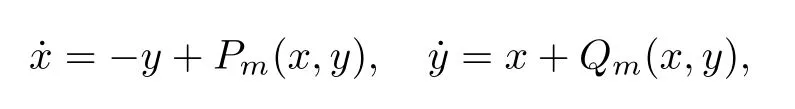
are known to be of center type,wherePmandQmare homogeneous polynomials of degreem(see [75,76]).There are very few results on the problem of the characterization of centers for polynomial systems of arbitrary degree(see [77,78]for Kukles homogeneous systems).Finally,we remark that the existence of invariant algebraic curves is closely related to whether center conditions for system(5.1)are verified,as is explained in [12,79].The center-focus problem has also been studied for three or higher dimensional systems by using symbolic or symbolicnumeric methods(see,e.g.,[80–82]).The classical result of Poincar´e and Liapunov introduced above has been recently extended to any finite dimensional integrable differential systems by Romanovskiand others [83].For a comprehensivepresentation of theresultson thecenter-focus problem,the reader is referred to the review articles [84,85].

6 Hopf Bifurcation of Small-Amplitude Limit Cycles

Consider planar differential systems of the form

wherePandQare real polynomials of degree at mostninxandy.Recall that a limit cycle of system(6.1)is an isolated periodic orbit of the system.The second part of Hilbert’s 16th problem [86]is concerned with the maximum number H(n)of limit cycles that system(6.1)can have.This problem is still open,even for the casen=2.Due to the work and effort of numerous researchers(see,e.g.,[66,87–96]),the lower and upper bounds on H(n)have been improved continuously.The following theorem exhibits some of the best results established in the literature:

Theorem 6.1([92–94,96–100])For planar differential systems of the form(6.1),the maximum number H(n)of limit cycles is≥4 and is individually finite forn=2.Moreover,H(3)≥13,H(4)≥20,H(5)≥28,H(6)≥35,and H(n)≥

For other developments related to H(n),we refer the reader to Li [101]and Han and Li [96].

The bifurcations of limit cycles may generally be placed into three categories:(1)Hopf bifurcation from a center or a focus;(2)Poincar´e bifurcation from closed orbits;(3)separatrix cycle bifurcations from a homoclinic or a heteroclinic loop.Selected results are presented here mainly for the first two categories of bifurcations,while the third category is comparatively more difficult,so far fewer techniques are available.

6.1 Bifurcation Methods

When the problem of studying limit cycles is restricted to the neighborhood of an isolated equilibrium,it reduces to the problem of studying Hopf bifurcations,which gives rise to the study of fine foci.The basic idea of constructing multiple limit cycles around an equilibrium is to compute the Liapunov constants and solve the coupled polynomial equations to find the conditions under which multiple limit cycles can bifurcate from the equilibrium.See [115,Chapter 3]for discussions on the efficiency of existing methods for computing Liapunov constants.

In addition to those based on Liapunov constants,there are several other methods that have been developed for studying the problem of Hopf bifurcations.These methods are based on the theories of normal forms [54,115],Melnikov functions [115,116]and time averaging [117–119].Various algorithms have been devised for the computation of normal forms [120,121,123]and the expansion of Melnikov functions near centers [116],but they giveno qualitative information about the limit cycles bifurcated.In contrast,using averaged functions,one can determine the shape of the bifurcated limit cycles up to any order in the parameterε(see,e.g.,[117,124]).On the other hand,it has been shown in [122]that the averaging method may be unable to detect possible limit cycles bifurcating from a Hopf bifurcation point,while the normal form theory can be used to overcome the difficulty.

6.2 Planar Differential Systems

When the origin of(5.1)is a fine focus of orderk,one may constructklimit cycles in the neighborhood of the origin by small perturbation.One may obtain conditionson the parameters for(5.1)to have a fine focus of orderkby solving the semi-algebraic system

The investigation of Hopf bifurcations was one of the early research directions exploring the applications of symbolic computation,and there is extensive work on it in the literature.Wang [102]first introduced symbolic-computational methods to studying the problem of limit cycles by constructing high-order fine foci,and provided a class of cubic differential systems with the origin as a fine focus of order 6 from which 6 limit cycles were constructed.Since then,a great amount of work on the interactions of differential equations with symbolic-computation has been carried out(see [11,16,103,107–110]).Li and Bai [103]and James and Lloyd [104]found particular classes of cubic systems with 7 or 8 small-amplitude limit cycles bifurcating from one fine focus.James and Lloyd’s systems were reinvestigated by Ning and others [105]to derive another condition under which 8 small-amplitude limit cycles may bifurcate.Yu and Corless [106]constructed a cubic system with 9 small-amplitude limit cycles by combining symbolic and numeric techniques.Later on,Lloyd and Pearson [111]reported more recent developments in handling very large computations involving resultants,and presented an example of a cubic planar polynomial system with 9 small-amplitude limit cycles surrounding a focus.Their example appears to be the first for which all the involved computations are performed symbolically(i.e.,exactly without numerical error).Chen and others [21]analyzed a cubic planar polynomial system based on the Liapunov constants for dynamical systems obtained by using normal form theory.In particular,they applied the methods of regular chains and triangular decomposition to the system and showed the computational efficiency of the methods.More recently,Yu and Tian [112]proved that planar cubic differential systems may have at least 12 small-amplitude limit cycles around an equilibrium;this is the best result known so far on the number of limit cycles around an equilibrium of cubic systems.Summarizing these results,we have the following theorem:

Theorem 6.2([21,102–104,112])There are families of cubic differential systems of the form(6.1)for which 6,7,8,9,12 small-amplitudelimit cyclescan bifurcatefrom an equilibrium.

More discussionson the Hopf bifurcation,as well as applications to practical problems from engineering and biological systems,can be found in [115,Chapters 4 and 5].

6.3 High-Dimensional Systems

In studying Hopf bifurcation of limit cycles for higher-dimensional systems,center manifold theory and normal form theory are two of the main tools(see,e.g.,[54,115,133]).Recently,the averaging method has been widely applied in the study of local dynamical behaviors of differential systems such as limit-cycle bifurcation and other more complex bifurcation analysis(see,e.g.,[117,118,124]).It turns out that the averaging method can not only determine the shape of the bifurcated limit cycles but also provide information on the stability of the limit cycles.

In what follows,we briefly explain the averaging method described in [126];it is used to deal with differential systems of the standard form

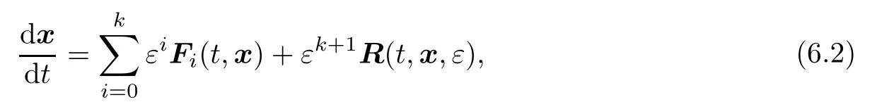
where Fi:R×D→Rnfori=0,1,···,kand R:R×D×(−ε0, ε0)→Rnare continuous functions and areT-periodic in the variablet,withDbeing an open subset of Rn,and where 0< ε0≪1 is a sufficiently small parameter.The averaging method works by defi ning a collection of functions fi:D→Rn,each fibeing called theith-order averaged function,fori=1,2,···,k,whose simple zeros control,for|ε|>0 sufficiently small,the limit cycles of system(6.2).

The process of using the averaging method to study limit cycles of differential systems consists essentially of three steps [119,Section 4]:(1)transform the considered differential system into the standard form of averaging(6.2)up to thekth order inε;(2)derive the symbolic expression of thekth-order averaged function fk(z);(3)determine the exact upper bound for the number of real isolated solutions of fk(z).More details about the averaging method can be found in [126,128,129].

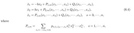
Now were call some of the existing results that are particularly relevant to Hopf bifurcations.Llibre and Zhang [117]proved that,up to the first order inε(i.e.,k=1),ℓ=2n−3limit cycles can bifurcate from the origin of a perturbed differential system in which the functions on the right-hand side are differentiable up to the third order,and that their Jacobian matrix at the origin has eigenvaluesε a±biandε csfors=3,···,n.They showed for the first time that the number of bifurcated limit cycles can grow exponentially with the dimensionn.Later on,Pi and Zhang [130]extended the result of [117]for differential systems with the functions on the right-hand side being differentiable from the third order to the(m+1)th order form>2,showing thatℓlimit cycles can bifurcate from the origin with eitherℓ≥mn−2/2 formeven orℓ≥mn−2formodd.This is the first result showing that the number of limit cycles from a Hopf bifurcation is a power function in the degree of the system.Recently,Barreira and others [131]proved thatℓlimit cycles can bifurcate from the origin withℓ=3n−2form=3,ℓ≤6n−2form=4,andℓ≤4·5n−2form=5.Other results on Hopf bifurcation of differential systems using the averaging method may be found in [118,124,125].

Huang and Yap [119]provided an algorithmic approach to analyze the bifurcation of smallamplitude limit cycles for planar differential systems of the form

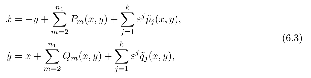
wherePm,Qmare homogeneous polynomials of degreeminxandy,are polynomials of degree at mostn2inxandy(usuallyn2≥n1≥2),and whereεis a small parameter.Assume that the unperturbed system(6.3)(i.e.,whenε=0)has a center at the origin.Using thekth-order averaging method,Huang and Yap gave an upper bound on the number of zeros of the averaged functions for the perturbed system(6.3)(see [119,Theorem 3.1]).More recently,Huang and Wang [127]studied perturbations of then-dimensional differential system

7 Bifurcation of Limit Cycles from Period Annuli

Consider planar differential systems of the form(6.1)with an equilibrium of center type.The set of periodic orbits surrounding the center is called its period annulus.A perturbation of the system usually breaks these periodic orbits but some of them might be maintained as limit cycles of the perturbed system.In this case,we say that limit cycles have bifurcated from the period annulus.

There are several methods for studying limit cycles bifurcating from the periodic orbits of a period annulus.These methods use different analytical tools:the Poincar´e return map [132],the Melnikov function [133],the averaging method [128,129]and the inverse integrating factor [134].Recently,some relationship between the method of Melnikov functions and the averaging method for studying the number of limit cycles bifurcating from the periodic orbits of planar analytical near-Hamiltonian differential systems was given in [135].

Now consider differential systems of the form

whereε >0 is a small parameter,andH,fandgare infinitely differentiable functions.Whenε=0,system(7.1)becomes a Hamiltonian system;thus it is called a near-Hamiltonian system.To introduce the Melnikov functions of arbitrary order,one must assume that the unperturbed system(7.1)ε =0has a family of periodic orbits,denoted byLh,which are defined by the level curveH(x,y)=hforh∈JwithJbeing an open interval.We first take a cross section,sayЦ,which is transverse to all of the periodic orbits inside the period annulus.Such a cross section can be constructed as follows:for any givenh0∈J,take a pointA0∈;then there exists a curve Ц passing throughA0and transverse to the periodic orbits of the unperturbed system(7.1)ε =0.

For anyhnearh0,the periodic orbitLhintersects the curveЦat a unique pointA(h)such thatH(A(h))=h.Note thatA(h0)=A0.Hence,we get a functionA(h):J→Ц,which has the same regularity as system(7.1).Consequently we can writeЦas

Now consider the positiveorbit of(7.1)starting atA(h).LetB(h, ε)denote the first intersection point of the orbit withЦ.It follows from(7.1)that

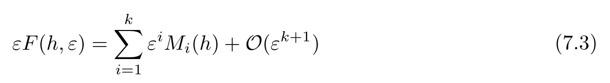
for any integerk≥1.The functionMiin(7.3)is usually called theith-order Melnikov function.It follows from(7.2)that

The following result gives a criterion for the existence of limit cycles of system(7.1):

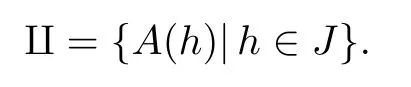
Lemma 7.1([135])Assume thatMk(h)/≡0 for somek≥1,and thatMj(h)≡0 forj=1,···,k−1.IfMkhas at mostmzeros onJ,taking multiplicity into account,then forε >0,a sufficiently small parameter system(7.1)has no more thanmlimit cycles bifurcating from the period annulus {Lh|h∈J}.

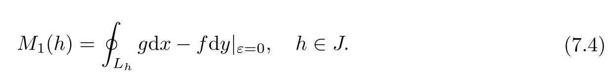
It is known that Arnold’s version of Hilbert’s 16th problem [136]is to study the maximum number of zeros of the Melnikov functionM1(h).The zeros ofM1(h)provide information on the persisting limit cycles of system(7.1)in the sense of the first-order Poincar´e bifurcation forεsufficiently small(see [137]).In the context of the weak Hilbert’s problem,the Lienard system

of type(m,n)is of special interest,whereare polynomials of degreesmandninx,respectively,and µ represents the parameters.System(7.5)is a special form of(7.1),withf(x,y, ε)=0,g(x,y, ε)=and the HamiltonianH(x,y)=it can be applied to model real-world oscillating phenomena(see [138]).

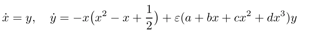
There are many interesting results on the bifurcation of limit cycles for Li´enard systems of the form(7.5)(see [22,139–142,145–147,152]and references therein).In the case when the degree of the HamiltonianH(x,y)is 4,Dumortier and Li [139]studied the Li´enard systems of type(3,2)profoundly,and obtained sharp upper bounds on the number of zeros of the corresponding Melnikov functions for 5 different cases.The main technique used in their study was to reduce the problem of bounding the number of limit cycles to that of studying the number of intersections of the related line with a curve by means of Picard–Fuchs equations and Riccati equations.For Li´enard systems of type(5,4)with symmetry,it has been shown that the dimension of the resulting Picard–Fuchs equations is the same as that of type(3,2)(see,e.g.,[140,141]).However,there may exist more than 3 generating elements of Melnikov functions when the Hamiltonian has a degree more than 4 without symmetry.In this case,the Picard–Fuchs equations and Riccati equations have higher dimensions,which increases the difficulty of investigating the intersections of the related plane and surface.There had been no result for type(4,3)until the Chebyshev criterion was introduced in [143,144].This algebraic criterion can deal with Melnikov functions with more than 3 generating elements for Li´enard differential systems(see,e.g.,[145,146]).In particular,Sun and Huang [22]proved that,by combining the regular chain theory and the Chevbyshev criterion,the perturbed system

has at most 6 limit cyclesbifurcating from the period annulus of the unperturbed system.Wang [147]showed that,by using interval analysis,the perturbed differential system

hasat most 6 limit cyclesbifurcating from the period annulus of the unperturbed one.These results have demonstrated again the feasibility and efficiency of symbolic-computational methods in studying the problems of limit cycles.However,in such studies,many manual interactions are still needed in the process of computation with algebraic systems.

Hu and others [148]proposed an algorithmic approach to automate the process of computational studies on the number of limit cycles that may bifurcate from a period annulus for Li´enard systems of the form(7.5).More precisely,they gave an algebraic criterion for the problem of determining whether the Melnikov function of the considered system has the Chebyshev property.This criterion has been reformulated as a problem of semi-algebraic system solving [36,37],to which available methods from polynomial algebra can be applied.

There is an interesting series of works on the number of zeros of Melnikov functions by the Chebyshev criterion(see [142,149]for type(5,4)and [150,151]for type(7,6)).However,the upper bounds obtained in almost all of the above-mentioned results are not the exact upper bounds(or sharp bounds).The sharp bounds are still open,even for Melnikov functions of Li´enard systems of type(4,3)(see two case studies in [152]).Exploring symbolic approaches to determine the sharp upper bounds on the number of zeros of Melnikov functions for certain types of Li´enard systems is a subject worthy of further study.

8 Symbolic Analysis of Biological Systems

Many biological networks are modeled mathematically as dynamical systems in the form of polynomial or rational differential equations.To understand biological phenomena described by complex dynamical systems,it is necessary to study their behaviors,such as stability,bifurcation,and limit cycles,qualitatively.Dynamical systems have signifi cant applications to biology,as shown by the pioneering application of game theory to evolution [153,154],and the introduction of deterministic chaos into ecology [155].

The general method outlined in Section 3 for equilibrium detection and stability analysis based on semi-algebraic system solving was proposed by Wang,Xia and Niu [16,41,156]initially for biological systems.It has been applied to the analysis of local stability and the bifurcation of limit cycles for several classes of systems of biochemical reactions [45,157].Niu and Wang [45]analyzed a cubic self-assembling micelle system with chemical sinks modeled by the dissipative dynamical system

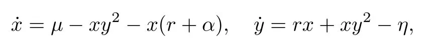
wherexandyare dimensionless concentrations of active free amphiphile and micelles,respectively.The rate coefficientsαandηrepresent chemical sinks for each species,andµandrare intrinsic parameters.All of the variables and parameters are positive.For such a concrete system,a complete classifi cation of the stability and types of equilibria in the hyperbolic case have been provided.Niu and Wang also obtained algebraic conditions on parameters for the occurrence of the three kinds of bifurcations(Hopf bifurcation,saddle-node bifurcation and Bogdanov-Takens bifurcation),and the stability and types of the bifurcation points.In particular,they demonstrated that 3 limit cycles can be constructed from a Hopf bifurcation point by small perturbation and the perturbed differential system remains polynomial.

Following the work of Wang and coauthors,many researchers have studied the problem of stability and bifurcation analysis with specialized techniques for efficient computation by taking the structures of the systems into account.The work of Shiu and Tang,with coauthors,was devoted to detecting equilibria of large-size biological networks with a special structure by using symbolic computation(see [160]for example).Hong and others [17]worked out a special algorithm for the stability analysis of a class of biological regulation systems MSRS,by exploiting the interesting structure of the differential equations.Sparsity is a common characteristic of many biochemical reaction networks.For a family of sparsepolynomial systems arising in chemical reaction networks,Gatermann and others [162,163]formulated the systems by graphs and showed that the solution structure of such systems is highly determined by the properties of the graphs.A considerable amount of work for sparse polynomial systems has been done(e.g.,on the number of real positive equilibria [162],the number of stable equilibria [163],and analysis of Hopf bifurcation [164])by considering the structure of the graphsbased on toric variety and using themethod of Gröbner bases.Mou and Ju [161]applied sparse triangular decomposition to analyze the equilibria of biological networks by exploiting the inherent sparsity of parameter-free systems via the chordal graph and by constructing suitable elimination orderings for parametric systems using the newly introduced block chordal graph.Sturm and Weber,with coworkers,used the QE method to detect the occurrence of Hopf bifurcations using reaction coordinates [158],and studied equilibria for some networks of large scale.In a more recent 11 author paper [159],the methods of virtual substitution,lazy real triangularization and CAD were used to analyze the equilibria and stability of two models of the mitogen-activated protein kinases(MAPK)cascade with 11 variables and 16 variables,respectively,and the conditions on the two unknown parameters for the systems to have 3 equilibria were established.More information about MAPK,as well as symbolic analysis of its multiple equilibria and bistability,can be found in [16,165,166].

In enzyme kinetics,a fundamental assumption is the so-called Quasi-Steady-State Assumption or Quasi-Steady-State Approximation(QSSA),which has a history of more than 90 years,and has proven to be very useful in analyzing the equations of enzyme kinetics.The idea of QSSA is simple:study the dynamics of the slow reactions,assuming that the fast ones are at a quasi-equilibrium,thereby removing such differential equations that describe the evolution of the variables at the quasi-equilibrium from the system.Li and others [169]proved,by using the qualitative theory of dynamical systems,that QSSA is always true in the simplest model with the second elementary reaction being irreversible,and that it may thus be called the Quasi-Steady-State Law(QSSL).Therefore,all conclusions based on QSSA now have a solid foundation in the irreversible case.Later on,Li [170]extended the application of QSSA in a more general model:the reversible one-substrate-one-product model.The application of QSSA in biochemical kinetics allows one to employ symbolic methods to simplify complex biochemical systems for the purpose of qualitative analysis.This kind of simplifi cation has been used in the study of metabolic processes and genetic regulation processes in system biology,which involves enzyme catalysis.For example,Boulier and coauthors applied differential elimination methods to deal with QSSA in order to perform reductions for biological models [172,173].They combined their method with reparameterization techniques to automate there duction of a family of models of genetic circuits and obtained conditions for the existence of Hopf bifurcation [171,174].

For the analysis of stability and limit cycles for population and epidemic models,especially Lotka–Volterra systems,Lu and coworkers performed an impressive amount of work by using methods of real solution isolation(see [108]for example).They also studied the problems of global stability analysis for several types of Lotka–Volterra systems [167,168]using Liapunov functions and the structure of Lasalle’s invariant set,together with Wu’s method of characteristic sets.Symbolic-computational methods have also been applied to qualitative analysis of dynamical systems in economy,control theory,systems science and other fields(see,e.g.,[175–178]).

9 Concluding Remarks

In view of the outcome of the research over the last three decades and the current state of the art,this survey has provided a brief account on how symbolic-computational methods have helped advancemodern research on the problem of the qualitative analysis of stability and bifurcations for systems of differential equations.The methods of symbolic computation have proven to be powerful in terms of their capability to solve algebraic and semi-algebraic systems and other related problems involving polynomial expressions of many thousands of terms.As the problems to be solved are posed usually with a theoretical or practical background,the solutions that may be found at the end of such large-scale computations are often concise and beautiful.Such computationally complex problems with conceptually simple solutions can be taken as ideal examples for illustrating and testing the applicability,efficiency,and limitation of sophisticated algorithms being developed to automate the process of mathematical problem solving.

Differential equationsappear almost everywhere in science and engineering.They have been used broadly to describescientific phenomena in biology,economics,control theory and complex networks.There are plenty of problems regarding the interaction between differential equations and symbolic computation that remain for further research and investigation.It is believed that symbolic and algebraic computation will continue playing an extremely important role in the development of the classical qualitative theory of differential equations.With Hilbert’s 16th problem underlined as an open challenge,advanced research supported with powerful methods of symbolic computation will certainly make the qualitative theory one of the most useful tools for automated problem solving in the field of differential equations and beyond.The reader is encouraged to make use of the tool to solveinteresting practical problems on hand,or to extend the tool significantly to tackle those problems which are currently intractable.

Acknow ledgementsThe first author wishes to thank Xianbo Sun for providing him with helpful references on recent developments regarding Li´enard systems.