Ensemble Numerical Simulations of Realistic SEP Events and the Inspiration for Space Weather Awareness

Chenxi Du,Xianzhi Ao,Bingxian Luo ,Jingjing Wang,Chong Chen,Xin Xiong,Xin Wang ,and Gang Li

1 National Space Science Center,Chinese Academy of Sciences,Beijing 100190,China;xzao@nssc.ac.cn

2 University of Chinese Academy of Sciences,Beijing 100049,China

3 Key Laboratory of Science and Technology on Environmental Space Situation Awareness,Chinese Academy of Sciences,Beijing 100190,China

4 State Key Laboratory of Space Weather,National Space Science Center,Chinese Academy of Sciences,Beijing 100190,China

5 School of Space and Environment,Beihang University,Beijing 100190,China

6 Department of Space Sciences,University of Alabama in Huntsville,AL 35899,United States of America

Received 2021 September 8;revised 2021 November 7;accepted 2021 November 9;published 2022 February 2

Abstract The solar energetic particle(SEP)event is a kind of hazardous space weather phenomena,so its quantitative forecast is of great importance from the aspect of space environmental situation awareness.We present here a set of SEP forecast tools,which consists of three components:(1)a simple polytropic solar wind model to estimate the background solar wind conditions at the inner boundary of 0.1 AU(about 20 R⊙);(2)an ice-cream-cone model to estimate the erupted coronal mass ejection(CME)parameters;and(3)the improved Particle Acceleration and Transport in the Heliosphere(iPATH)model to calculate particle fluxes and energy spectra.By utilizing the above models,we have simulated six realistic SEP events from 2010 August 14 to 2014 September 10,and compared the simulated results to the Geostationary Operational Environmental Satellites(GOES)spacecraft observations.The results show that the simulated fluxes of＞10 MeV particles agree with the observations while the simulated fluxes of＞100 MeV particles are higher than the observed data.One of the possible reasons is that we have adopted a simple method in the model to calculate the injection rate of energetic particles.Furthermore,we have conducted the ensemble numerical simulations over these events and investigated the effects of different background solar wind conditions at the inner boundary on SEP events.The results imply that the initial CME density plays an important role in determining the power spectrum,while the effect of varying background solar wind temperature is not signi ficant.Naturally,we have examined the in fluence of CME initial density on the numerical prediction results for virtual SEP cases with different CME ejection speeds.The result shows that the effect of initial CME density variation is inversely associated with CME speed.

Key words:Sun:coronal mass ejections(CMEs)–Sun:particle emission–acceleration of particles–shock waves–methods:numerical

1.Introduction

Solar energetic particle(SEP)events are hazardous space weather events caused by solar activities.SEPs may include electrons,protons,and heavy ions from both the solar and the interplanetary medium,and their energies can range from keV to GeV.The start of a solar proton event(SPE)is de fined as the time when the first three consecutive data points of the 5 minutes averaged integral flux of＞10 MeV protons observed by the Geostationary Operational Environmental Satellites(GOES)equal or exceed the 10 proton flux unit(1 pfu=1p/[cm2·s·sr])threshold (Zhong et al.2019).The first observation of SEP event in human history was reported by Forbush(1946).SEP events are historically arranged into two categories:impulsive and gradual(Cane et al.1986;Reames 1995,1999),corresponding to different observational characteristics.The particles time-intensity pro file of an impulsive event shows the characteristic of a short-term(within a few hours)“pulse”in the observation,while the pro file of a gradual event usually tends to be characterized by long periods(about two days or even longer).The two categories are often intertwined(Cane et al.2004;Tylka et al.2005;Li and Zank 2005)in an actual physical evolution.Generally,most SEP events possess gradual features(Reames 2013).From the physical mechanism point of view,it is widely accepted that impulsive SEP events are originated in the solar flare regions,while the SEPs of gradual events are accelerated through the Diffusive Shock Acceleration(DSA)process(Reames 1994,1996,1997).The idea of the DSA mechanism was explored by Axford et al.(1977),Krymskii(1977),Blandford&Ostriker(1978),and Bell(1978a,1978b)to explain the supernova shock acceleration process of the galactic cosmic rays,and summarized by Drury(1983).

Since SEP events are signi ficant threats to space and airborne systems and astronauts in orbits,many efforts have been made toward the development and the application of SEP forecast methods in the past decades.Several models are used to predict the crucial parameters of SEP events(including duration,peak intensity,onset time and probability)based on remote sense data,solar events,and in situ measurements(Alberti et al.2017;Anastasiadis et al.2017;Balch 1999,2008;Cohen et al.2001;Engell et al.2017;Kahler et al.2007;Laurenza et al.2009;Núñez 2011;Posner 2007,2009).These models mainly fall into two categories:the traditional statistical(or empirical)models and the emerging arti ficial intelligence(machinelearning)models.In addition,a series of numerical simulations for SEP events that are caused by CME-driven shocks have been carried out(Zank et al.2000;Li et al.2003,2012;Luhmann et al.2010,2017;Linker et al.2019;Hu et al.2017).

Zank et al.(2000)proposed a dynamic onion-shell model for studying particle acceleration and transport in the heliosphere,which was further developed and known as the PATH(Particle Acceleration and Transport in the Heliosphere)model by Li et al.(Li et al.2003;Li and Zank 2005)and Rice et al.(2003).The PATH model is a comprehensive one-dimensional numerical model,which has been continuously improved over the past decades(Zank et al.2006,2007;Li et al.2012;Verkhoglyadova et al.2012,2013,2015).Hu et al.(2017)has extended the PATH model to the improved Particle Acceleration and Transport in the Heliosphere(iPATH)model,which includes a 2D con figuration.In the iPATH model,characteristics of the shock evolution and energetic particle acceleration are calculated in a 2D plane,and the distribution function of energetic particles at any location in the computational domain is obtained through the 2D transport module.The application of the iPATH model in previous works(Hu et al.2018;Fu et al.2019;Ding et al.2020)has shown the effectiveness of the model.However,the prediction of realistic SEP events is still far more beyond the scope of those theoretical literatures.

We attempt in this paper to present a feasible tool sets that can be used to predict SEP events.The tool sets,driven by the observed solar wind condition data from the Advanced Composition Explorer(ACE)satellite or from other spacecraft at 1 AU and the CME coronagraph data from the Solar and Heliosphere Observatory(SOHO),include:(1)a polytropic model for estimating background solar wind parameters at 0.1 AU(about 20R⊙);(2)an ice-cream-cone model for inverting CME parameters;(3)a model for particle acceleration and transport(improved Particle Acceleration and Transport in the Heliosphere:iPATH).We have performed numerical simulations on six realistic SEP events observed by GOES satellites using the tool sets,and have furtherly investigated the in fluence of various initial conditions on the energy spectra adopting the ensemble experiments.At the latter of this paper,we have computed the effect of the CME initial density on the numerical prediction results for virtual SPEs with different CME ejection speeds.

2.The SEP Forecast Tool Sets

In general,very high energy particles in an SEP event caused by a large CME can arrive at the Earth within 30 minutes after the CME eruption,and the SEP event can last for several days.Upon obtaining the 1 AU solar wind conditions and the CME parameters,the tools sets are able to compute the particle flux and spectrum near the Earth for space weather forecasters to determine whether or not an SPE warning should be issued.Figure 1 illustrates the schematic of the SEP event forecast procedure.In this method,we average the solar wind data(including solar wind velocity,plasma temperature,plasma number density and magnetic field strength)observed by the ACE satellite,and feed them into the 1D polytropic model(Fu&Hu 1995)to calculate the background solar wind parameters at the inner boundary(0.1 AU,about 20R⊙).In addition to the initial background solar wind parameters at the inner boundary,the iPATH model also requires CME eruption parameters as initial conditions.As described in the upper right side of Figure 1,based on the white-light coronal images observed by the Large-Angle Spectrometric Coronagraph(LASCO)onboard the SOHO spacecraft at Lagrangian point L1,the icecream cone model utilizes an inversion algorithm to obtain the CME parameters(including CME ejection speed,CME source location,and CME angular width)(Xie et al.2004).We use the iPATH model to numerically simulate the SEP event with the parameters of both background solar wind and CME.The output includes SEP fluxes and energy spectra.

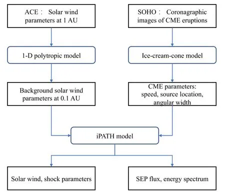
Figure 1.Schematic of the SEP event forecast procedure.

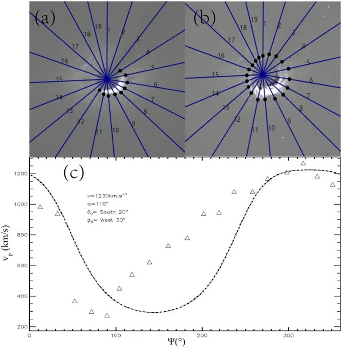
Figure 2.Manual CME front detection and the ice-cream-cone model fitting result of the SEP event occurred on 2014 April 18.In panels(a)and(b),the numbered blue lines cover the projected angular width of the CME,and the black dots on the blue lines represent the CME front marked manually.In panel(c),the triangle represents the derived projected velocity for each position angle selected by manual detection,and the dotted line represents the fitting result;v represents the fitted CME ejection speed;αrepresents the fitted angle width;(θ0,φ0)represents the fitted longitude and latitude of the source location.

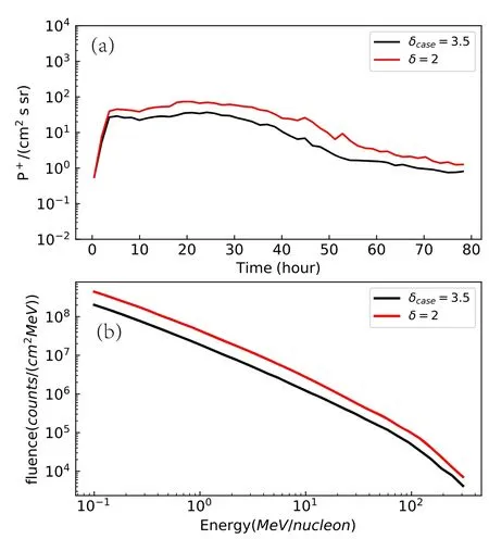
Figure 3.Comparisons of the simulated fluxes(≥10 MeV)and the eventintegrated energy spectra betweenδ=3.5 andδ=2.In panel(a),the red line represents the simulated flux forδ=2,and the black line represents the simulated flux forδ=3.5;in panel(b),the red and black lines represent the event-integrated energy spectra forδ=2 andδ=3.5,respectively.

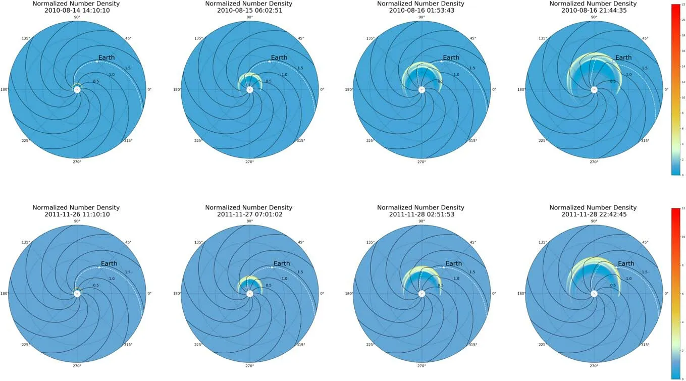
Figure 4.The simulated propagation of the CME-driven shock in the ecliptic plane.From(a)to(f)are the ordered results of the six events listed in Table 1.The white star in each subplot marks the Earth;the solid spiral lines depict the IMF,and the dashed white line is the magnetic f ield line passing through the Earth;the color bar denotes the normalized number density

The iPATH model,in which the ZEUS-3D(V3.5)code is embedded,simulates the background solar wind,the CMEdriven shock,and the associated particle acceleration and transport in a 2D computational domain.The calculation of the iPATH model is sequently performed by three steps:the first step is to simulate the background solar wind;the second step is to introduce a disturbance in the background solar wind to generate a CME-driven shock and construct a 2D“onion-shell”to calculate the particle acceleration at the shock front;and the third step is to calculate the transport of the solar energetic particles accelerated by the shock in the interplanetary space.In fact,simulating CMEs and the associated shock waves is rather complicated and computational resource consuming,and is one of the frontier subjects in space weather.However,the scope of this paper is not to understand the sophisticated CME internal structures.Instead,we focus on the particle acceleration and transport upstream and downstream of the shock front.The DSA mechanism states that the characteristics of the leading CME-driven shocks and the ambient turbulence are the determining factors in forming SEP events and the CME internal structures are almost irrelevant.Therefore,for simplicity the way we drive the shock in the second step is to launch a blast wave at the inner boundary to mimic a CME.The 2D onion shell constructed in the second step and the corresponding calculation of particle acceleration and transport are the main improvements to the previous 1D PATH model.In the 2D iPATH model,the total diffusion coef ficientκis given by Li et al.(2012)

whereκ‖andκ⊥are the parallel and the perpendicular diffusion coef ficients,respectively;θBNis the angle between the shock normal and the interplanetary magnetic field(IMF).

Evidently,θBNvaries along the shock front and the total diffusion coef ficient changes accordingly,which one-dimensional con figuration cannot reveal.Due to the existence of perpendicular diffusion,it is expected that an object in space may experience a flux enhancement even if it is not connected to the shock front by the IMF lines directly.Considering the perpendicular diffusion coef ficient in a 2D onion shell con figuration(see Hu et al.2017 for more details)enables us to compute the cross-field diffusion effect scattering the energetic particles into a wider longitudinal range.The accelerated energetic particles then escape near the shock and propagate outward along the interplanetary magnetic field lines.During this process,the energetic particles are scattered by the interplanetary turbulence.The particle transport is controlled by the focused transport equation,and the third step of the iPATH model uses a Monte Carlo method to solve it.

ZEUS-3D is a non-relativistic magnetohydrodynamics(MHD)solver written in FORTRAN,which uses staggered grids and upwind scheme.The MHD equations to be solved are

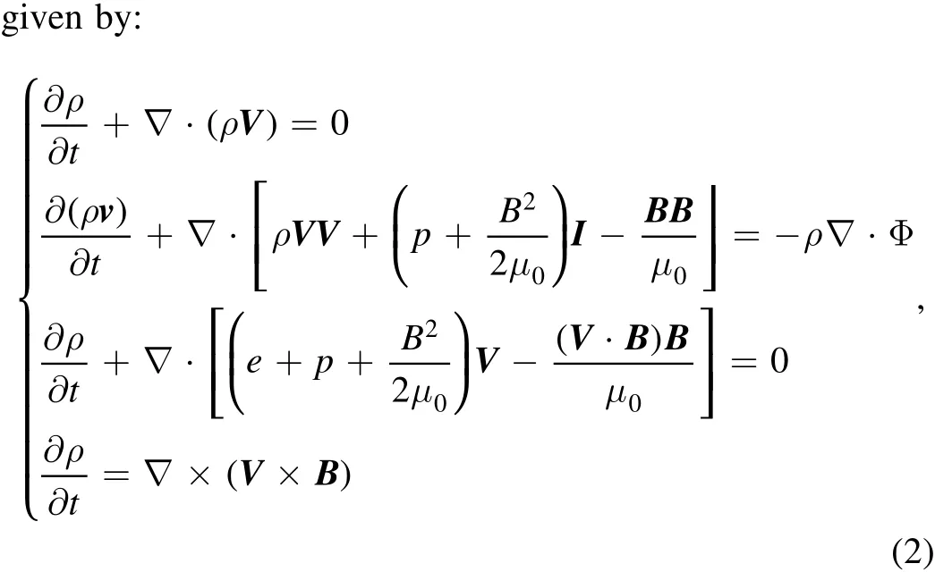
whereρis the fluid density;V is the velocity of the fluid;pis the thermal pressure of the fluid;B is the magnetic field strength;eis the total energy of per unit volume,including the internal energy and magnetic energy;andΦis the gravitational potential.

ZEUS-3D itself has the ability to solve MHD equations in 3D space while it is simpli fied to solve equations in a 2D space in this paper.Only a finite number of grids are selected in the third dimension in the iPATH model,i.e.,only one plane(θ=90°:an approximation to the equatorial plane or eclipticplane)is retained to solve the MHD equations.Although this approach makes the iPATH model lose the ability to solve 3D problems,it can save computational resources and reduce the computation time signi ficantly.Thus,the numerical simulation can be completed in a short time after the eruption of a CME,and hence provides a timely warning.

The iPATH model takes 0.1 AU(about 20R⊙)as the inner boundary,and a period of disturbance(blast wave)is introduced at the inner boundary to initiate a CME.Both the initial density and the speed disturbance over the inner boundary are not uniform and obey a Gaussian distribution along the azimuth.The background solar wind parameters(solar wind velocity,magnetic field strength,plasma temperature,and density)at the inner boundary and the CME parameters(angular width,ejection speed,and disturbance duration)are necessary parameters to drive the model.In the 2D computational domain of the numerical simulation,1500 grids are distributed evenly along the radial distance from 0.1 AU to 2 AU,and 360 grids are distributed evenly along the azimuth.The initial magnetic field in theiPATH model is the Parker-spiral field(Parker 1958),which is given by:

whereBris the radial component of the magnetic field;Bφis the tangential component of the magnetic field;B0is the magnetic field strength at the source location ofR=R0;Ωis the angular velocity of the Sun;USWis the solar wind speed andθis the elevation in the spherical coordinate system.

Certain criteria must be made to choose proper SEP cases in order to investigate the effect of various inner boundaries on the prediction results.First,the selected event can be regarded as an isolated case,i.e.,no other obvious events occur in a certain time before and after the selected event.Therefore,there is no apparent in fluence of other events on the simulation results.Second,the selected events better possess different ejection speeds,so that we can investigate the SEP events caused by CME driven shocks with different strength.Third,the ejection direction of the selected events should not deviate the ecliptic plane too much(≤30°).

We have picked six gradual SEP events from 2010 August to 2014 September for the ensemble simulation,using the observations of Geostationary Operational Environmental Satellites(GOES)data as the reference.The associated CME events are all relatively isolated,and their eruption source locations are all within 30°latitudinally.The eruption speed of these CME events range from 970 km s-1to 1310 km s-1.The background solar wind parameters at 1 AU are determined from 24 h average solar wind data observed by the ACE satellite before the events.We revert the CME eruption parameters using the ice-cream-cone model.Figure 2 shows the manual CME front detection and the ice-cream cone model fitting result of the event occurred on 2014 April 18.Figures 2(a)and(b)show the detection procedure of the CME front from SOHO/LASCO C3 images.The fitted results are presented in Figure 2(c),and the estimated CME speed is 1230 km s-1with an angular width of 110°(see details in Wang et al.(2018)for more information about the fitting procedure).

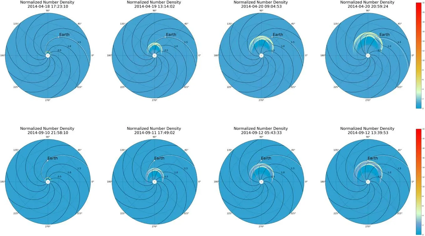
Figure 4.(Continued.)

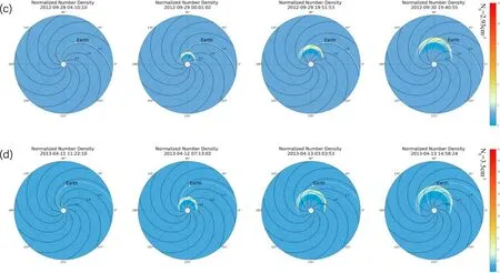
Figure 4.(Continued.)

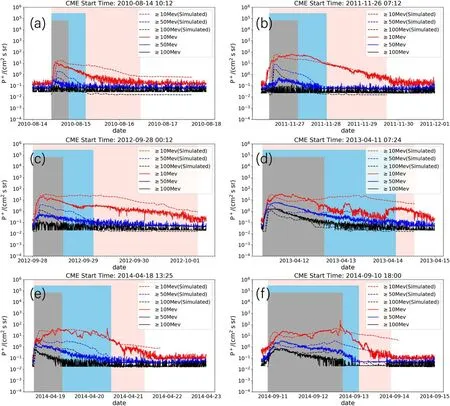
Figure 5.Comparisons between the observed unidirectional integrated flux by GOES satellite and the simulated results.The red,blue,and black curves represent the flux of energetic protons with energy ranges≥10 MeV,50 MeV,and 100 MeV,respectively;the solid lines and the dashed lines represent the results of GOES observations and numerical simulations,respectively.The pink,blue,and gray color blocks cover the time windows from the beginning to the recovery state of the flux with the energy ranges≥10 MeV,50 MeV,and 100 MeV,respectively.The time windows are manually selected.

For simplicity,we assume that the inner boundary conditions along the inner boundary are axisymmetric when calculating the background solar wind parameters,i.e.,all points have identical physical quantity at the inner boundary.Table 1 shows the obtained inner boundary parameters for all the six events.The first column is the date of the selected SEP events,the same as those in the list provided by CDAW Data Center(https://cdaw.gsfc.nasa.gov/CME_list/sepe/).The second to the sixth columns are the solar wind parameters(solar wind velocity,magnetic field strength,number density,and plasma temperature)at the inner boundary,and the seventh to the ninth columns are the CME eruption parameters(ejection speed,angular width and source location)calculated by the ice-creamcone model.It is noticeable that the IMF consists of two components,namely the radial component(Br)and the tangential component(Bφ).

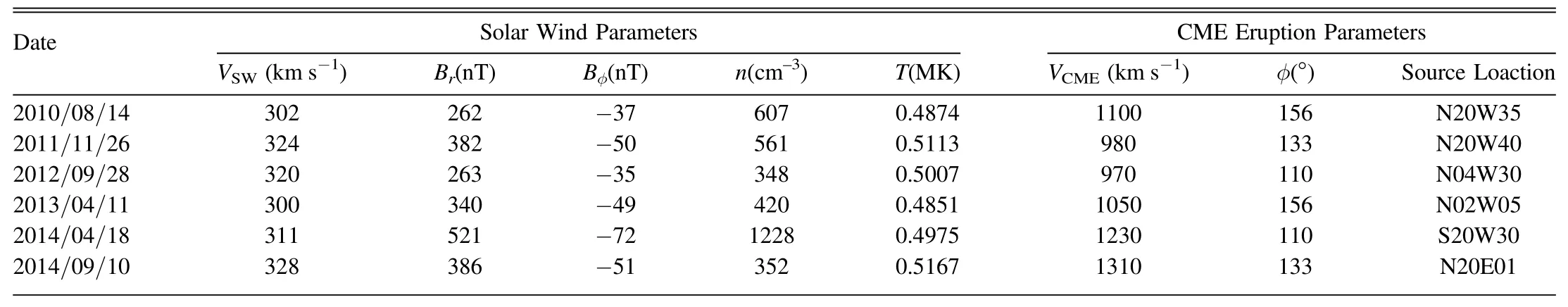
Table 1Inner Boundary Conditions at 0.1 AU(～20 R⊙)

In the iPATH model,the particle injection rate is given by Verkhoglyadova et al.(2015)

whereE0is the particle injection energy under the condition of a parallel shock;is the injection energy under the condition of an oblique shock,which is a function of the angle between the normal direction of the shock and the magnetic field line;(-δ)is the power-law exponent of the distribution function of the seed particle energy spectrum;χis the injection ef ficiency,which is in a range of not more than 1%.In this paper,we have selected properχvalues for each of the six events to fit simulations and observations better.

Li et al.(2012)usesδ=3.5 in their simulations.The source of the seed particles may come from the solar wind suprathermal tail.Observations show that the power-law like spectral index for heavy ions in the ambient medium prior to the arrival of the shocks is in the range of 1～3.5(Desai&Mason 2004).We may adopt these numbers in our SEP simulations.Both the simulated flux(≥10 MeV)and the energy spectrum ofδ=3.5 are compared to those ofδ=2.0.Because a harder power-law index indicates more seed particles with higher energies enter the diffusive shock acceleration process,it is evidently that both the flux and the energy spectral intensity of the latter are higher,as shown in Figure 3.On the other hand,due to the different acceleration ef ficiency for moderate-energetic particles and high-energetic particles,the power spectrum tends to be softer in the case ofδ=2.0.We useδ=3.5 in the rest of the paper.

Figure 6.Comparisons of CME-driven shock propagations with different inner boundary background solar wind temperatures.The white star in each subplot marks the Earth;the solid spiral lines depict the IMF,and the dashed white line is the magnetic f ield line passing through the Earth;the color bar denotes the normalized number densityThe coef f ciient before T represents the multiple factor of the original temperature.

3.Results

We present in this section the simulated results for the six gradual SEP events given in Table 1 as well as the ensemble simulation results.

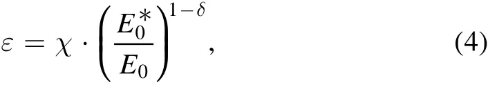
Table 2The Value ofσfor the Three Time Windows in Figure 5

3.1.Event Simulation Results

Figure 4 shows the propagation of the CME-driven shocks in the ecliptic plane at four different time steps.The colorbar illustrates the normalized number density,which is de fined byis the number density;Ris the radial distance;N0is the averaged number density of the background solar wind at distanceR0,which is taken to be 1 AU.Each row corresponds to an SEP event in Table 1.Figure 4(a)shows the simulated event that occurred on 2010 August 14.The CME start time is 10:12 UT,and the arrival time at the Earth of the simulated shock is about 21:44:35 UT on 2010 August 16.Figure 4(b)shows the simulated event on 2010 November 26.The CME start time is 07:12 UT,and the arrival time at the Earth of the simulated shock is about 22:42:45 UT on 2010 November 28.Figure 4(c)shows the simulated event on September 28,2012.The CME start time is 00:12 UT,and the arrival time at the Earth of the simulated shock is about 19:40:55 UT on 2012 September 30.Figure 4(d)shows the simulated event on 2013 April 11.The CME start time is 07:24 UT,and the arrival time at the Earth of the simulated shock is about 14:58:24 UT on 2013 April 11.Figure 4(e)shows the simulated event on 2014 April 18.The CME start time is 13:25 UT,and the arrival time at the Earth of the simulated shock is about 20:59:24UT on 2014 April 18.Figure 4(f)shows the simulated event on 2014 September 10.The CME start time is 18:00 UT,and the arrival time at the Earth of the simulated shock is about 19:39:53 UT on 2014 September 10.Since the SEPs experience pitch angle scattering along the IMF lines,the position at the shock front where the magnetic field line connects the Earth,which sometimes is called the cob point(IMF connecting the observer point)is crucial for the particle flux that the Earth may intercept.Figure 4 shows a shock gradually transforms from a quasi-parallel state to a quasiperpendicular state in the process of the evolution as the connecting point moves along the shock front.The shock obliquity at the cob point is effected by both the shock evolution and the cob point connectivity.Noting that the source locations of the two events occurred on 2013 April 11 and 2014 September 10(see in Figures 4(d)and(f))are slightly different from the rest four events that occurred on the west side,both events erupted near the meridian.Because of this,and also due to the Parker spiral,in Figures 4(d)and(f),the cob point on the shock front is at the shock edge at the beginning of the CME eruption,and then gradually moves close to the shock center when the shock arrives at the Earth.

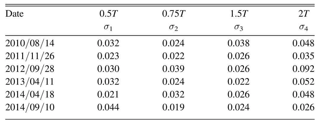
Table 3The Values ofσin Figure 7

Figure 6.(Continued.)

Figure 5 compares the simulated unidirectional integrated fluxes at the Earth to the observations made by GOES 13 or GOES 15.In fact,the CMEs erupt near the solar surface rather than at the inner boundary of the model at 0.1 AU.Indeed,the results of the iPATH model ignore the acceleration process within the distance from the actual eruption location to 0.1 AU.In order to compare the simulated results to the observations,we have made some adjustments to the start time of the simulated SEP events by adding a time shift,which is estimated by the CME ejection speed and the distance of the inner boundary from the eruption source surface,i.e.,the time that the CME travels to 0.1 AU since it forms.To estimate the disagreement between the simulation results and the GOES observations,a parameterσis introduced for quantitative analysis and is de fined as the following(Wu&Qin 2018):

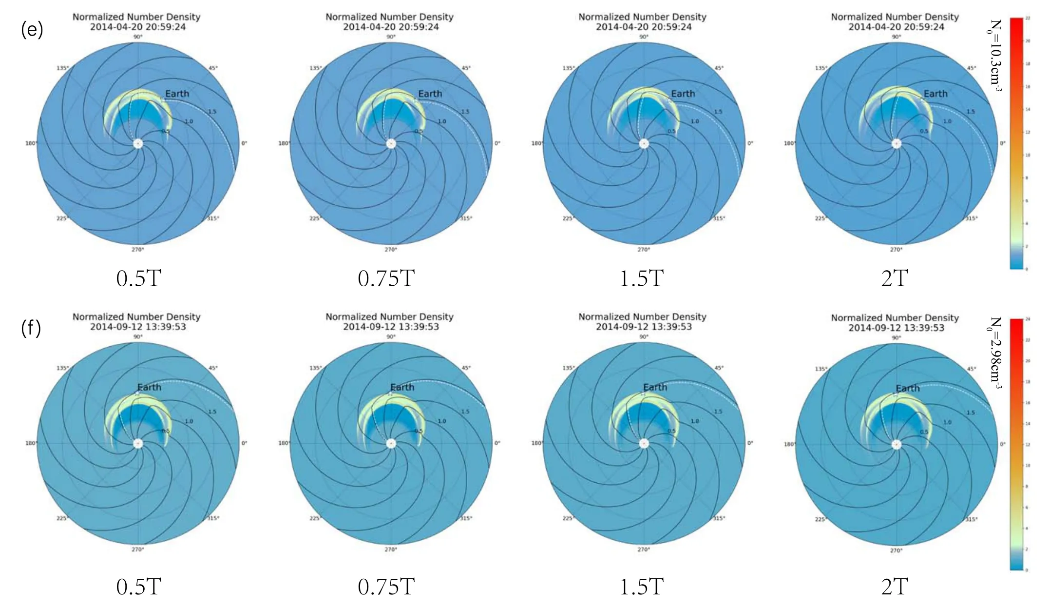
Figure 6.(Continued.)

whereF(E)andf(E)are the energy spectra to be compared.

Since the SEP flux of different energy range bears different declining phase(see Figure 5),we have manually selected three time windows,corresponding to the flux enhancement pro file for the energy ranges≥10 MeV,50 MeV,and 100 MeV,respectively.In the gray window,the value ofσ for energy ranges≥10 MeV,50 MeV,and 100 MeV is calculated and denoted byσ1,σ2andσ3in Table 2,respectively.In the blue window,the value ofσfor energy ranges≥10 MeV and 50 MeV is calculated and denoted byσ4andσ5in Table 2,respectively.In the pink window,theσfor the energy range≥10 MeV is calculated and denoted asσ6in Table 2.Theσvalue can be used to estimate the relative degree of agreement for different energy levels.The results in Table 2 show that in the gray window,the simulated results can re flect the observed flux better in the energy range of≥10 MeV than those in the energy ranges of≥50 MeV and 100 MeV(the smaller theσ,the better the result).In the blue window,expect for the third and fourth events,the simulated results for the energy range of≥10 MeV agree with the observations slightly better than those for the energy range of≥50 MeV.Finally,σ for the energy range of≥10 MeV in the pink window demonstrates the overall agreement between the simulation results and the GOES observations.Noting the complexity of SEP events and due to the extremely lack of observational data,it can be regarded as a good agreement if the deviation of the computed fluxes from the measured ones is within a magnitude of one order,i.e.,σ＜1.0 on an average.Theσvalues in Table 2 indicate that the simulated≥10 MeV fluxes agree with the observations well,while the simulated≥50 MeV and≥100 MeV fluxes need improvement.

The results in Figure 5 and Table 2 indicate that the simulated flux given by our tool set re flects the observation better in the energy range of≥10 MeV than those in the energy range of≥100 MeV and higher.One of the possible reason is that the particle injection rate in the higher energy range is higher in simulation than that in the actual physical process.Another possibility is that our 2D numerical simulation yields a higher shock compression ratio than the realistic 3D con figuration.It is interesting that in Figure 5(f),the proton flux possesses a bimodal structure.As mentioned before,the movement of the cob point at the shock front plays a crucial role in the formation of proton fluxes.In fact,there are two signi ficant factors in this procedure.One is that the compression ratio decreases with the shock evolution process(accompanied by the weakening of the shock strength),which makes the proton flux have a downward trend;the other is that the compression ratio at the shock center is higher than that at the shock edge,which makes the proton flux increases as the cob point moves to the shock center.The final proton flux is a tangled result of these two factors.Obviously,the second factor is dominant in Figure 5(f).

The reasons and theories behind three s popularity are numerous and diverse. The number has been considered powerful across history in different cultures and religions, but not all of them. Christians67 have the Trinity, the Chinese have the Great Triad (man, heaven, earth), and the Buddhists68 have the Triple Jewel (Buddha, Dharma, Sanga). The Greeks had the Three Fates. Pythagoras considered three to be the perfect number because it represented everything: the beginning, middle, and end. Some cultures have different powerful numbers, often favoring seven, four and twelve.Return to place in story.

Figure 7.Comparisons of event-integrated energy spectra with different inner boundary background solar wind temperatures.Black lines represent the cases of the original temperatures,and the red lines represent the cases with varied temperatures.σis calculated with Equation(5).

Figure 8.Comparisons of CME-driven shock propagations with different initial CME densities.The white star in each subplot marks the Earth;the solid spiral lines depict the IMF,and the dashed white line is the magnetic f ield line passing through the Earth;the color bar denotes the normalized number densityThe coef f icient before n represents the multiple factor of the original density.

3.2.Ensemble Simulation Results:Temperature Variation

In general,the solar wind temperature at the inner corona cannot be measured directly.However,we can estimate this quantity by physical models.In our SEP forecast tool sets,we calculate the inner boundary solar wind temperature through a 1D polytropic model.No doubtly,this method may overestimate the solar wind temperatures.In order to evaluate the impact of inaccurate temperature estimation on the SEP prediction,we adopt different background solar wind temperatures at the inner boundary for our ensemble experiments.

Figure 6 shows the snapshots of the CME-driven shocks in the ecliptic plane with four different inner boundary background solar wind temperatures illustrated by the normalized number density at the same time step(it is the time when the shock arrives at the Earth in Figure 4).Figures 6(a)–(f)correspond to the six events listed in the first column of Table 1(in the same order).We set the temperature to 0.5,0.75,1.5,and 2 times of the original value(the sixth column of Table 1)as the inner boundary background solar wind temperatures,respectively.From Figure 6,there are almost no obvious changes with different temperature conditions.The shock travels slightly faster with a higher temperature setting.

Figure 7 compares the event-integrated energy spectra of the ensemble cases(with the ampli fication factor equal to 0.5,0.75,1,1.5,and 2,respectively)to the original con figuration.As shown in Figure 7,the variations of the spectra with different inner boundary background solar wind temperatures are insigni ficant.Similarly,to quantify these variations,the parameterσis used to indicate the disagreement between the two energy spectra,the values ofσin Figure 7 are listed in Table 3.

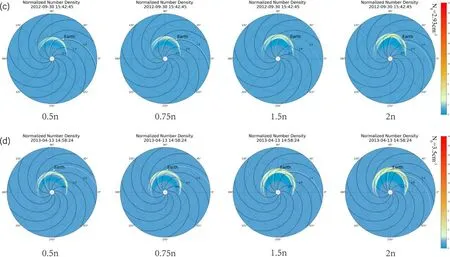
Figure 8.(Continued.)

All theσvalues in Table 3 are less than 0.1,which is consistent with the statement that the impact of varying inner boundary solar wind temperature on SEP events is insigni ficant.

3.3.Ensemble Simulation Results:Density Variation

In our tool sets,the initial maximum CME density at the center is simply calculated by multiplying the background solar wind by a ratior,which is given by:

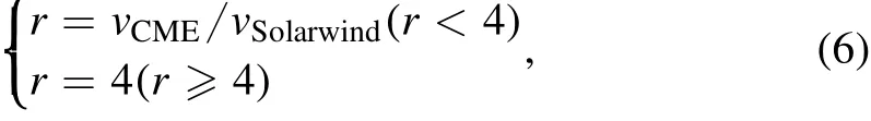
Figure 8 shows the snapshots of the CME-driven shocks in the ecliptic plane with four different initial CME densities at the same time step.Figures 8(a)–(f)are the six events(in the same order as shown in Table 1).In this subsection,we set the density to 0.5,0.75,1.5,and 2 times of the original value(calculated from the fifth column of Table 1 by multiplying the ratior)as the inner boundary initial CME densities,respectively.As shown in Figure 8,we can see that in all events,the position of the shock has a relatively obvious change,and the shock travels faster with a larger initial CME density.

Figure 9 shows the comparisons of the event-integrated energy spectra of the ensemble cases(with the ampli fication factor equal to 0.5,0.75,1,1.5,and 2,respectively)to the original con figuration.The correspondingσis listed in Table 4.Compared to Figure 7,the effect of the initial CME density is more signi ficant than that of the background solar wind temperature.It is noticeable that theσin Figures 9(a),(e)and(f)is signi ficantly smaller than that of the rest,which implies that the variation of the initial CME densities has less effect on these three events.Because these three events have larger ejection speed,it can be inferred that the impact of the variation of the initial CME densities will decrease as the CME ejection speed increases.Therefore,we further investigate the in fluence of CME initial densities on the numerical prediction results with different CME ejection speeds.

Keeping the rest parameters unchanged,we have tested 10 evenly distributed speeds in the range from 1310 km s-1to 2210 km s-1as the CME ejection speeds.The simulated results with the conditions of the original CME density and 0.5 times the original CME density are calculated for comparison.Figure 10 depicts the variation ofσwith different CME ejection speeds.It can be quantitatively shown that the effect of changing the initial CME density on the simulation results of SEP events is inversely associated with the CME ejection speeds(which is normalized byv0=1000 km s-1).A function in the form ofy=ax+bis used to linearly fit the distribution ofσ,and the result of least square fitting gives thata=-0.15 andb=0.41.

Figure 8.(Continued.)

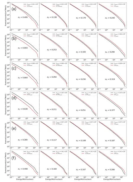
Figure 9.Comparisons of event-integrated energy spectra with different initial CME densities.Black lines represent the cases of the original densities,and the red lines represent the cases with the varied densities.σis calculated with Equation(5).

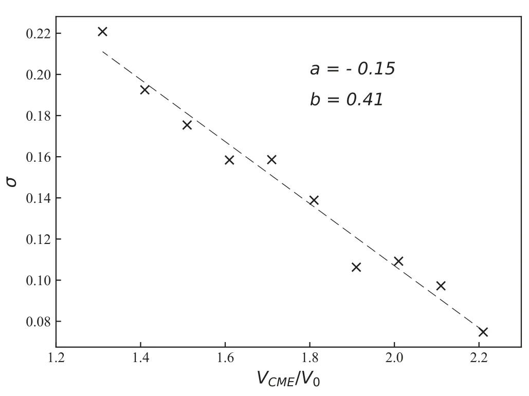
Figure 10.The dependence ofσon CME ejection speeds.The black dashed line indicates the linear least square fit.

4.Discussion

We have simulated six gradual SEP events from 2010 August 14 to 2014 September 10 using our SEP event forecast tool sets.The quantitative comparison between the numerical simulation results and the GOES observations shows that the numerical simulation results of the energetic particle flux with energy≥10 MeV are in better agreement with the observations than those of the energetic particle flux with energy≥50 MeV or≥100 MeV.

A simple 1D polytropic model is implemented in the SEP forecast tool sets to estimate the background solar wind parameters at the inner boundary.In general,it is easier to estimate the speed,density,and magnetic field of the background solar wind at the inner boundary than to estimate the temperature.The temperature estimated by the 1D polytropic model is often higher than the actual temperature.Additionally,the effect of background solar wind temperature on SEP events is rarely discussed in previous literatures.Therefore,we have conducted a research over the effect of background solar wind temperature on SEP forecast by means of the ensemble test.The numerical results show that the shadow thrown by inaccurate background temperature on the SEP forecast near the Earth is almost negligible.Clearly,as long as the temperature of the background solar wind near the inner boundary lies in a rational range,the SEP forecast will not be altered signi ficantly.This conclusion is of great value in space environmental situation awareness when providing supports for space projects and missions.

On the other hand,it is very complicated to estimate the density spatial distribution among the CME bulk.This paper has quantitatively studied the effect of the initial density of CMEs over the energy spectra of SEP events with ensemble simulations.The results show that higher CME initial density leads to a faster shock and a higher energy spectrum intensity.The higher CME initial density also leads to a slightly harder energy spectrum.On this basis,we further investigate the dependence of the effect on CME ejection speed.The dependence appears to be quasi-linear and inversely associated.

At present,our SEP forecast tool sets have been deployed at the Space Environment Prediction Center(SEPC;Liu&Gong(2015))of NSSC,CAS,and are able to provide services for the safeguard of the near-Earth satellites and the deep-space exploration missions.This is the first version of our SEP forecast tool sets and there are still many aspects to be optimized:(1)how to obtain accurate inner boundary conditions;(2)implemention of a 3D CME simulation;(3)how to determine a more realistic injection rate.It is also very meaningful to further test our tool sets against other spacecraft observations in the future:Venus Express,MAVEN,PSP,and Solar Orbit to name a few.

Acknowledgments

Acknowledgements We acknowledge the use of NOAA GOES data(https://satdat.ngdc.noaa.gov/),the ACE data from the ACE Science Center(www.srl.caltech.edu/ACE/ASC.Use of ZEUS-3D,developed by CLARKE D A.at the ICA(www.ica.smu.ca with support from NSERC,is acknowledged.This work is supported by the National Science Foundation of China(No.42074224),the Key Research Program of the Chinese Academy of Sciences,grant No.ZDRE-KT-2021-3,and Pandeng Program of National Space Science Center,Chinese Academy of Sciences.

ORCID iDs

Bingxian Luo https://orcid.org/0000-0002-7762-2786 Xin Wang https://orcid.org/0000-0003-1735-6233