A novel combination belief rule base model for mechanical equipment fault diagnosis
Mnlin CHEN, Zhijie ZHOU, Bngcheng ZHANG, Gunyu HU,You CAO
a High-Tech Institute of Xi’ an, Xi’ an 710025, China
b School of Applied Technology, Changchun University of Technology, Changchun 130000, China
c Guangxi Key Laboratory of Trusted Software, Guilin University of Electronic Technology, Guilin 541004, China
KEYWORDS Fault diagnosis;Belief rule base;Directed acyclic graph;Evidential reasoning;Mechanical equipment
Abstract Due to the excellent performance in complex systems modeling under small samples and uncertainty,Belief Rule Base(BRB)expert system has been widely applied in fault diagnosis.However, the fault diagnosis process for complex mechanical equipment normally needs multiple attributes, which can lead to the rule number explosion problem in BRB, and limit the efficiency and accuracy. To solve this problem, a novel Combination Belief Rule Base (C-BRB) model based on Directed Acyclic Graph (DAG) structure is proposed in this paper. By dispersing numerous attributes into the parallel structure composed of different sub-BRBs,C-BRB can effectively reduce the amount of calculation with acceptable result. At the same time, a path selection strategy considering the accuracy of child nodes is designed in C-BRB to obtain the most suitable submodels. Finally, a fusion method based on Evidential Reasoning (ER) rule is used to combine the belief rules of C-BRB and generate the final results.To illustrate the effectiveness and reliability of the proposed method, a case study of fault diagnosis of rolling bearing is conducted, and the result is compared with other methods.
1. Introduction
With the rapid development of science and technology, the scale of equipments or systems has become more and more huge and complex, and the probability of faults during operation process is also increasing. If the faults cannot be found and handled in time, it will influence the system and cause accident.Therefore, fault diagnosis has become a significant research direction to achieve the safety and reliable operation of mechanical equipment.In current studies, the fault diagnosis method for mechanical equipment can be divided into four categories:
(1) The analysis-based method. It analyzes the mechanism of the research object, and explores the operation rules and features.The analytical-based method obtains the internal relationship between the relevant features and the faults, and finally expresses it by establishing a mathematical model.For example, by analyzing various fault mechanisms of motor drive system, Huang et al. proposed a motor drive system fault classification method based on improved hidden Markov model, and achieved good results.Shen et al. proposed a pure torsional dynamic model of planetary gear considering wear, and used the model to analyze the vibration of planetary gear.Although the analytical-based method can effectively and accurately determine the faults, it requires definite mathematical description which is difficult to be obtained in practical engineering.
(2) The data-driven method. It is mainly constructed based on the model which needs lots of data to realize selflearning.For example, Li et al. proposed a fault diagnosis model of rolling bearing based on the improved deep belief network with PSO algorithm, which realizes the recognition of bearing running states.Wang et al.proposed a Back Propagation (BP) neural network based model as the guidance technology of fault diagnosis, which constructed a fast automatic fault diagnosis system.Although the above researches have achieved good experimental results,the data-driven method lacks effective utilization of qualitative expert knowledge,which makes it unable to deal with the small sample problem.In addition, most data-driven methods belong to the ‘‘black box modeling”, which lack interpretability for the diagnosis results.
(3) The knowledge-based method. It is essentially the process of infusing new or unknown knowledge from the existing knowledge, which is mainly represented by expert systems.Li et al. proposed an expert system of fault diagnosis for flight simulator,which gets a better performance.Yang et al.proposed an expert system of fault diagnosis for gear box in wind turbine,which could diagnose five faults.Although the expert system can obtain the better result of fault diagnosis, it is based on fault tree analysis normally, which leads to complex structure,and deficiency of quantitative data processing ability.
(4) The semi-quantitative information method. It can make use of both qualitative knowledge and quantitative data.Belief Rule Base (BRB) is one of the typical methods that can handle the various uncertainty, ambiguity,and semi-quantitative information, and has been widely applied in the field of fault diagnosis. Another advantage of BRB model is high interpretability and small sample processing capacity because of its transparent reasoning process and effective supplement of expert knowledge to data-driven process.For example, Lv et al. used BRB in the fault diagnosis of flight control system, and realized efficient and reliable diagnosis under small sample conditions.Feng et al. used BRB with attribute correlation to model complex systems and realize high-precision fault diagnosis of oil pipeline.Cheng et al. proposed a BRB fault diagnosis method with mixed belief,and carried out feasibility verification under various fault models of high-speed train drive device.However, in current studies, the fault diagnosis methods based on BRB can only be applied under the condition that small number of features are extracted. When more features need to be considered,the number of belief rules in BRB will grow exponentially,which makes parameter optimization become very difficult, and is easy to fall into local optimum.To solve this problem, Chang et al. proposed a BRB structure learning method based on PCA, which reduced the number of features and completed the construction of BRB in the case of multiple features.However, these features from PCA are non-interpretable, which undermines the practicability of BRB applications.
It can be seen in the above analyses that the existing fault diagnosis methods all have some limitations. In the field of mechanical equipment fault diagnosis, the problem will become challenging. Most mechanical equipment are constantly moving, and the parts are interacted with each other.Therefore, fault features contain a variety of uncertain information, and the data samples are hardly to be obtained. As mentioned above, BRB is very suitable for fault diagnosis of mechanical equipment. However, there is still a difficulty that needs to be solved. Compared with other systems, the fault characterizations of mechanical equipment are more complex,and most of characterizations are persistent signals, such as vibration and temperature, which can extract large number of features for fault diagnosis.Thus,limited by the complexity of the model, it cannot diagnose the fault accurately.
To solve the problem, a novel Combination Belief Rule Base (C-BRB) model based on Directed Acyclic Graph(DAG) structure for fault diagnosis of mechanical equipment is proposed in this paper.DAG is derived from the graph theory, which denotes a graph with directions on edges but no loops.It is often used to describe the process of a project or system, and easy to understand and implement.Hu et al. used DAG to establish a BRB classification model(DAG-BRB) for network intrusion detection.In this paper,the thought and the structure of the proposed C-BRB are different from DAG-BRB. In DAG-BRB, BRB model is divided into several binary classification models, where the number of attributes does not change. In C-BRB, BRB model is divided into several sub-BRBs, each of which only has a part of attributes.
The innovations of the manuscript can be concluded as follows. First, a novel C-BRB model is proposed to generate a decomposed BRB model with fewer attributes, which can easily embed the expert knowledge into the model, and each sub-BRB in the proposed C-BRB model can be well trained to generate more accurate results.Second,a parallel optimization process of C-BRB model is proposed to solve the problem of massive parameter optimization.
The remainder of this paper is organized as follows.In Section 2, relevant problems of fault diagnosis model based on BRB are described.The C-BRB model is proposed in Section 3.In Section 4, the fault diagnosis process based on C-BRB is designed, and an optimization process is proposed. In Section 5, the rolling bearing simulation data are taken as a case to verify the effectiveness of the proposed method, and the cross validation method and comparative experiment are used to verify its reliability and advantage. Section 6 is a summary of this paper.
2. Problem formulation
In the fault diagnosis process of complex mechanical equipment, we often face some problems. For example, although the observable signals of mechanical equipment(such as vibration signals)have a large number of sampled data,the patterns that can reflect the failure of the equipment are limited. After the feature extraction,the number of the obtained useful samples is small.Therefore,how to make full use of expert knowledge to make up for deficiency of samples during the model training is an urgent problem to be solved. Another problem is how to effectively describe all kinds of uncertain information. During the process of mechanical equipment fault diagnosis, there are various kinds of uncertain information in the collected data such as randomness, fuzziness, ignorance, and so on. Describing these uncertain information comprehensively can reflect the real states of the equipment more objectively.
The above problems can be solved effectively by the BRB model because of its ability to effectively utilize the expert knowledge and multiple types of uncertain information.BRB is an expert system that is developed based on the traditional If-Then rules, which was firstly proposed by Yang et al. in 2006.The weights of each feature and rule are considered in the rule construction, and the belief degree is added to the Then part of the rule. BRB has the ability to model nonlinear data with fuzzy uncertainty, probability uncertainty, and ignorance.The general description of BRB is as follows:

However,there are still some problems to be solved in BRB model for fault diagnosis of mechanical equipment.
Problem 1. As mentioned above,the signal of complex mechanical equipment can be used as the input of BRB after feature extraction. When the number of these features increases, the scale of BRB will increase exponentially. Thus, it is difficult for experts to set the initial BRB parameters. For example, in a BRB model with 3 attributes, each of which has 4 referential levels, the number of the rules is 64. When the number of attributes increases to 10,the number of the rules will increase to 1048576. As such, it is impossible for experts to embed knowledge into the model.
Problem 2. The increase of BRB scale also brings great pressure for model optimization.A large number of parameters will make the dimension of the solution space increase,and the high-dimensional optimization is very easy to fall into the local optimal solution, which leads to the increase of calculation amount and the decrease of precision.
To address the above challenge,this paper proposes a Combination BRB model (C-BRB) under multiple features. For a more detailed description of C-BRB, see Sections 3 and Section 4.
3. Establishment of combination belief rule base model
To solve the challenges mentioned in Section 2, a novel Combination Belief Rule Base (C-BRB) model for mechanical equipment fault diagnosis is proposed in this paper. By dispersing numerous attributes into the parallel structure composed of different sub-BRBs with Directed Acyclic Graph(DAG), C-BRB can effectively reduce the amount of calculation with acceptable results. The framework of C-BRB model consists of two parts: (A) Establishment of DAG-based combination BRB structure, and then determining the optimal path in combination BRB structure. (B) Fusion of results by Evidential Reasoning (ER) rule. The implementation process of the proposed C-BRB fault diagnosis algorithm is described in detail as follows.
3.1. Framework of fault diagnosis model
The structure of the proposed C-BRB model is composed of two parts,as shown in Fig.1.In part I,the monitoring signals collected by the sensors are used to extract features according to the feature system of the equipment operation state. Then,according to the feature combination rule, multiple sub-BRBs are constructed as the vertex sets of DAG structure.Afterwards, each sub-BRB can be trained independently to obtain the better result, which is used as the weight of the arc between two sub-BRBs. Finally, the related algorithm is used to traverse the vertexes and arcs of the DAG to obtain an optimal path.The vertexes(that is,the set of sub-BRB represented by V) on the optimal path can cover all the features and have high accuracy. In part II, each sub-BRB in the optimal path is fused to obtain the final fault diagnosis results.
3.2. C-BRB based on DAG structure
(1) Establishing the DAG structure.DAG is composed of a number of vertexes and weighted directed edges connecting each vertex,usually expressed as G=(V,E,W).V is a set of vertexes, and each vertex could denote an activity of system. E is a set of directed edges, and each edge from one vertex (parent vertex) to another vertex (child vertex),called arc,means that after the execution of one activity,the next activity begins to execute.Multiple arcs from a parent vertex can point to multiple child vertexes.Multiple arcs from multiple vertexes may also point to the same child vertex. The execution of the activity represented by a child vertex is determined by one of its parent vertices. W is a set of weight of directed edges, and represents the cost of performing the next activity. In the DAG, starting at the first vertex (the source point),connections are arced from vertex to vertex in the order in which the activities are executed.In DAG,starting at the first vertex(the source point),arcs are used to establish vertex-to-vertex connections in the order in which activities are executed. Finally, a number of arcs and vertexes formed from the source point of a number of paths, representing a variety of execution processes to complete a task in a system.The C-BRB model is based on DAG.Therefore,the establishment of C-BRB model requires the construction of DAG first, and the process is as follows:

Fig. 1 Fault diagnosis model framework based on DAG and BRB.
Step 1.Feature extraction is carried out from the vibration signal of mechanical equipment,and then the obtained features are sorted.The sorting principle is determined according to the specific type of mechanical equipment. Finally,the feature set is established.
Step 2. The first n (n = 2 or n = 3) features are selected from the feature set to build the initial sub-BRB (a BRB that consists of a part of features) which is according to the construction rules of BRB and combined with expert knowledge. It is the first vertex of the DAG, namely, the source point.
Step 3.Starting from the source point,as the parent vertex,child vertexes are generated downward with the same number of features in the parent vertex. Each child vertex consists of one feature from the parent vertex and n-1(n=2 or n=3)unused features selected in order from the feature set.At the same time,an arc from the parent vertex to each child vertex is established.
Step 4.With each child vertex as the parent vertex,the child vertex continues to be generated, and the composition of the child vertex is consistent with that described in Step 3,until the features in the feature set have been used once.At this point, all the DAG has been built.
It should be noted that in the generation process of DAG,all vertexes except the source point are created by their parent vertexes, which means that these vertexes are dependent on each other. The process can be shown in Fig. 2.
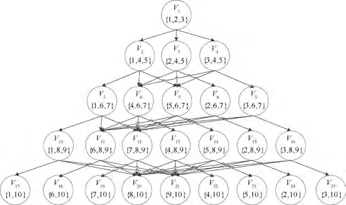
The finished DAG looks like an upside-down tree. However, the edges of DAG are not attached with weights. Fig. 3 shows the unweighted DAG built according to the process shown in Fig. 2 with the 10 features. It has a total of 25 vertexes,among which,the first 16 vertexes are composed of 3 features,while the last 9 vertexes are composed of 2 features,since there is only 1 feature in the feature set that has not been used.
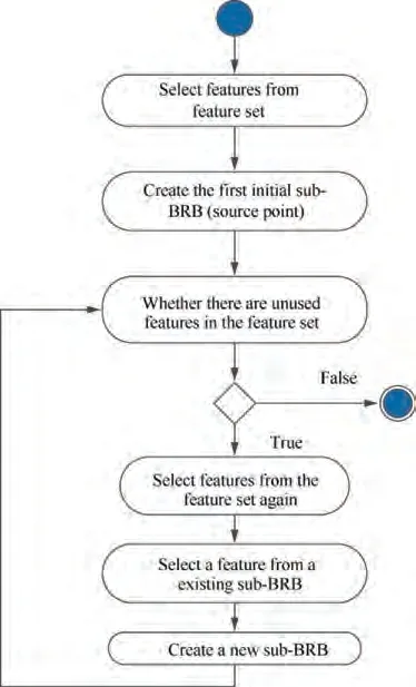
Fig. 2 Establishing process of DAG.
In Fig. 3, f(i=1,2,...,10) is the ith feature, which is selected from the feature-ordered feature set. Circles 1-25 denote 25 sub-BRBs,which can be also regarded as 25 vertexes of DAG.Except for the source point 1,the combination form of the features within 2-25 vertexes are determined by the features of its parent vertex and unused features in feature set.At the same time,since 2-25 vertexes belong to child vertexes,arcs from the parent vertex to each child vertex are established respectively. The directed edges between the parent vertexes and child vertexes are arcs of DAG, of which no weights are set. After the set of vertexes is obtained, the weight of the arc is determined by the sub-BRB accuracy of the end point of the arc, which can be calculated by the training process of BRB. Suppose that a sub-BRB is composed of M features,and eis the input monitoring data of quantitative form of the ith feature. It is necessary to represent eas the form of belief distribution based on the criteria set by the expert knowledge.If A(i=1,2,...,M;j=1,2,...,J)is the referential value of the ith feature,j is the number of possible referential values.γis the numerical representation given by experts to each referential value. αindicates the belief degree of the input value ecompared to γ. Thus, ecan be converted to αby the following equation:

The value of αcan be calculated as follows:
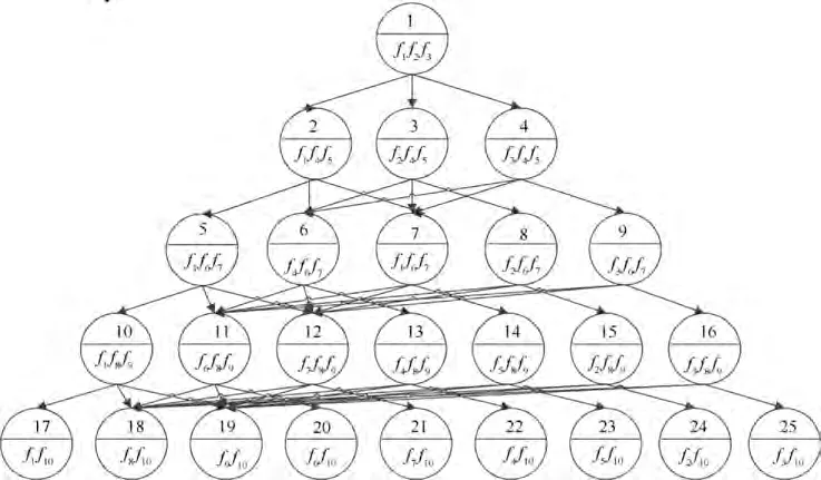
Fig. 3 Unweighted DAG with six features.
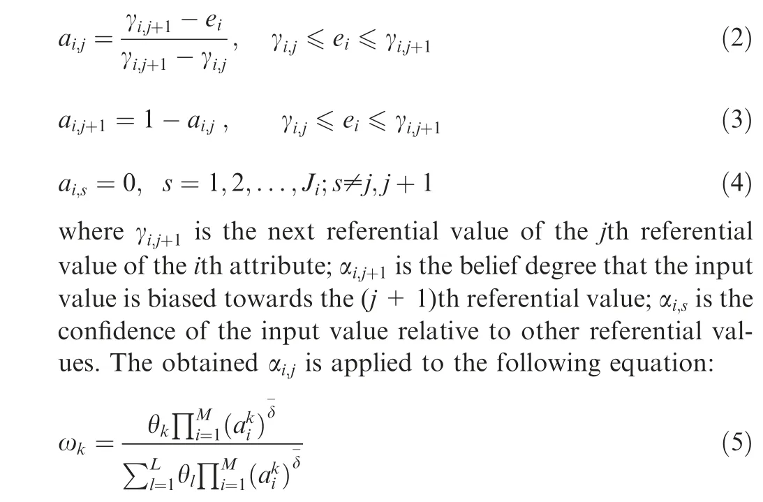
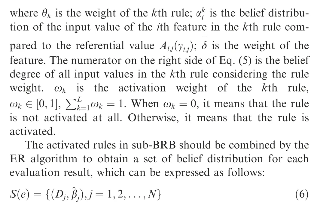
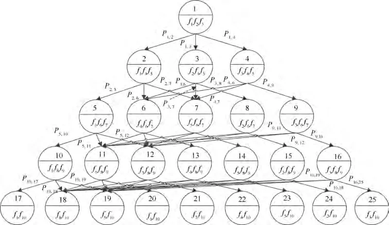
Fig. 4 DAG with six features.
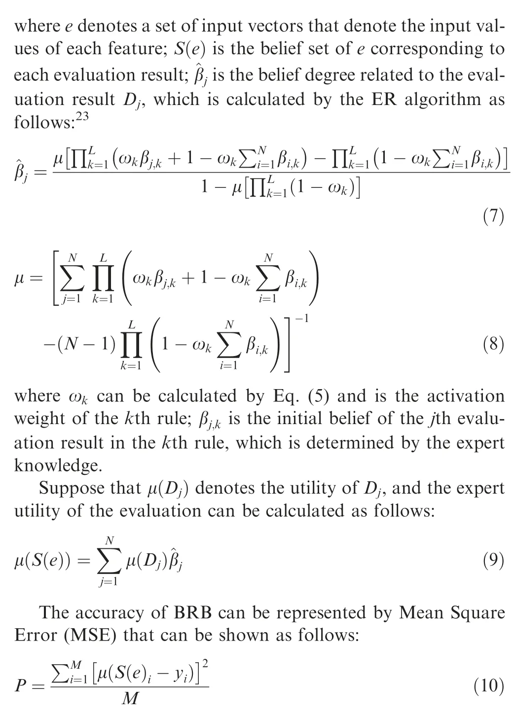
where P denotes the MSE,which also denotes the weight of the arc;M denotes the number of rules in one BRB;μ(S(e))is the utility of R;yis the actual result of R.Thus,a complete DAG is constructed. The weight of arcs is added to Fig. 3 to obtain the DAG as shown in Fig. 4.
In Fig.4,Pis the weight of arc that is from the ith vertex to the jth vertex.Due to the page space constraints,the weights of arcs with vertexes 6,7,8,11,12,13,14 and 15 as parent vertexes pointing to their respective child vertexes are not indicated in Fig. 4. But in fact, these weights need to be calculated. In addition, since the fact that some of the parent vertexes produce partial sub-vertexes is coincident, their arcs that point to the child vertexes have the same weight. For example, vertex 2 and 3 have the same child vertex 6 and 7,and then P=P,P=P.
It is important to note that there is a correlation between vertexes during the creation of vertexes, but each sub-BRB can be performed independently when calculating the weights.This is because each sub-BRB is an independent feature set after the DAG is built. During weight calculation, only the relationship among its own internal features is considered,without considering the features of other sub-BRBs. For this reason, each sub-BRB can be optimized and calculated separately, and all sub-BRBs can be calculated and optimized in parallel computing environment. This makes C-BRB model have high execution efficiency.
(1) Getting the optimal set of sub-BRBs. In the DAG, the smaller the arc weight is, the higher the accuracy of the end BRB will be.Therefore,the shortest path to findshould be assigned the minimum sum of weights from the source point to the lowest vertex. It can ensure full coverage of features and high accuracy of results. For the structure of DAG, there are many algorithms that can generate the smallest sum of weights, such as Dijkstra algorithm, Floyd algorithm and so on.In this paper, Dijkstra algorithm is used to obtain the shortest path. Taking the example of DAG as shown in Fig. 4,the basic process is introduced.

Table 1 Matrix Mfor DAG.
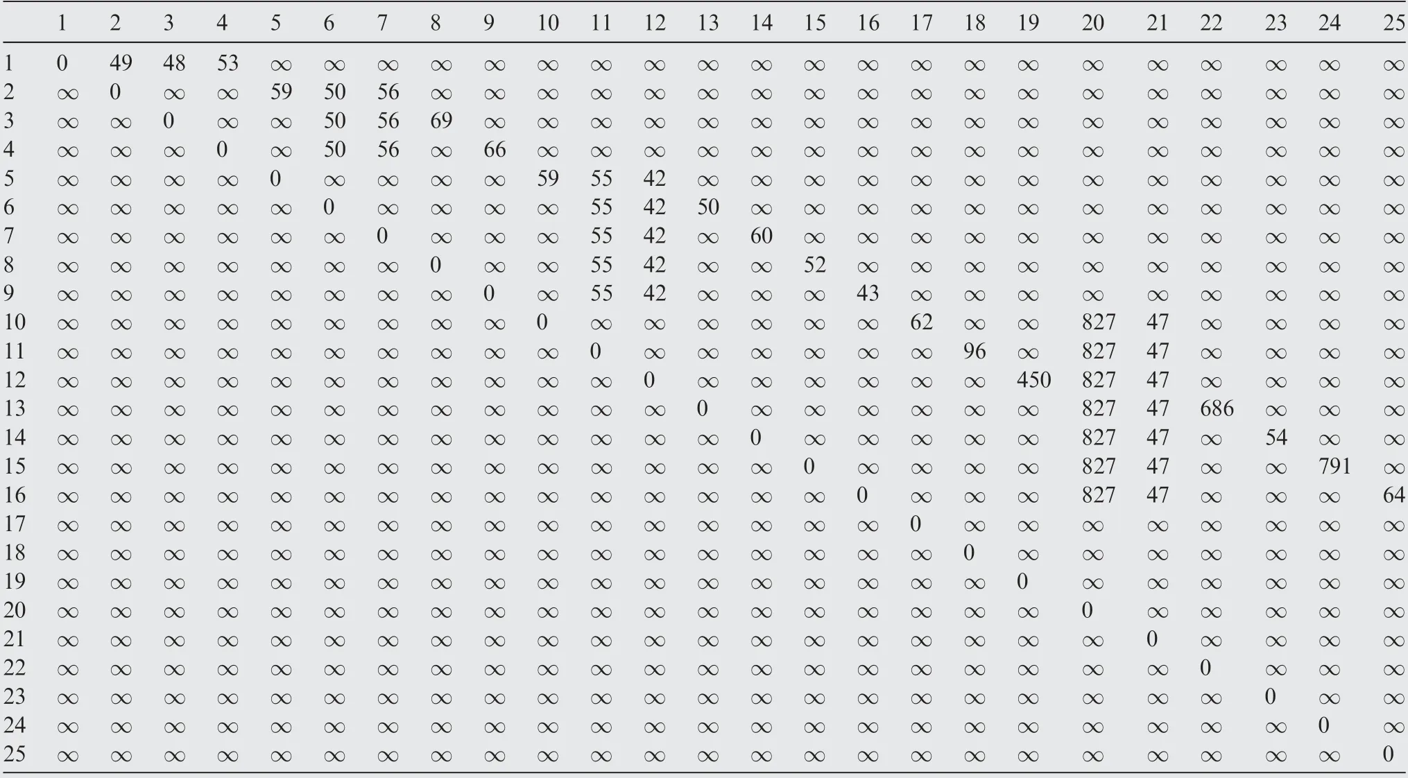
As shown in Fig. 4, let DAG be (V,E,W), where V={1,2,3,4,5,6,7,8,9,10,11,12,13,14,15,16,17,18,19,20,21,22,23,24,25}is the set of vertexes,E={<1,2>,<1,3>,<1,4>,<2,5>,<2,6>,<2,7>,<3,6>,<3,7>, <3,8>,< 4,6 >,< 4,7 >,< 4,9 >,< 5,10 >,< 5,11 >,< 5,12 >,<6,11>,<6,12>,<6,13>,<7,11>,<7,12>, <7,14>,<8,11>,<8,12>,<8,15>,<9,11>, <9,12>,<9,16>,< 10,17 >,< 10,18 >,< 10,19 >,< 11,18 >, < 11,19 >,< 11,20 >, < 12,18 >, < 12,19 >,< 12,21 >,< 13,18 >,< 13,19 >, < 13,22 >, < 14,18 >,< 14,19 >,< 14,23 >,< 15,18 >,< 15,19 >, < 15,24 >,< 16,18 >, < 16,19 >,< 16,25 >} is the set of arcs, W = {P,P,P,P,P,P,P,P, P,P,P,P,P,P,P, P,P,P,P,P,P,P, P,P,P,P, P,P,P,P,P,P,P,P, P,P,P,P,P,P,P,P,P,P,P,P,P,P} is the set of the weights of arc. According to the above analysis,the matrix M can be constructed,as shown in Table 1, and we set V, as shown in Eq. (11):

In Table 1, the row label is the start point of the arc. The column label is the end point of the arc. The elements in each row are the weight of the arc from the start point to the end point. Since the arcs of DAG are unidirectional, the values on the diagonal are all 0. The Vis the set of vertexes on the shortest path. Initially, there is only source point 1.
The following is an example of finding the shortest path by traversing the first 9 vertexes.According to the matrix M,there are three arcs from source point 1 to vertex 2, 3, 4, and the weights are P,P,P. Suppose that Pis the minimum,namely, the weight of the arc from source point 1 to vertex 2 is the minimum,and then vertex 2 is filled into V.At this time,V={1,2}. Then, the weights of arcs from source point 1 to vertex 2, 3, 4 are summed with the weights of vertexes 2, 3, 4 to their child vertexes 5,6,7,8,9 respectively.The sum results are put into the matrix M,and then the set Vis updated by the vertex of the path with the minimum sum of weights.The process can be shown as follows:
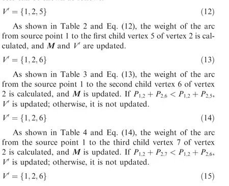
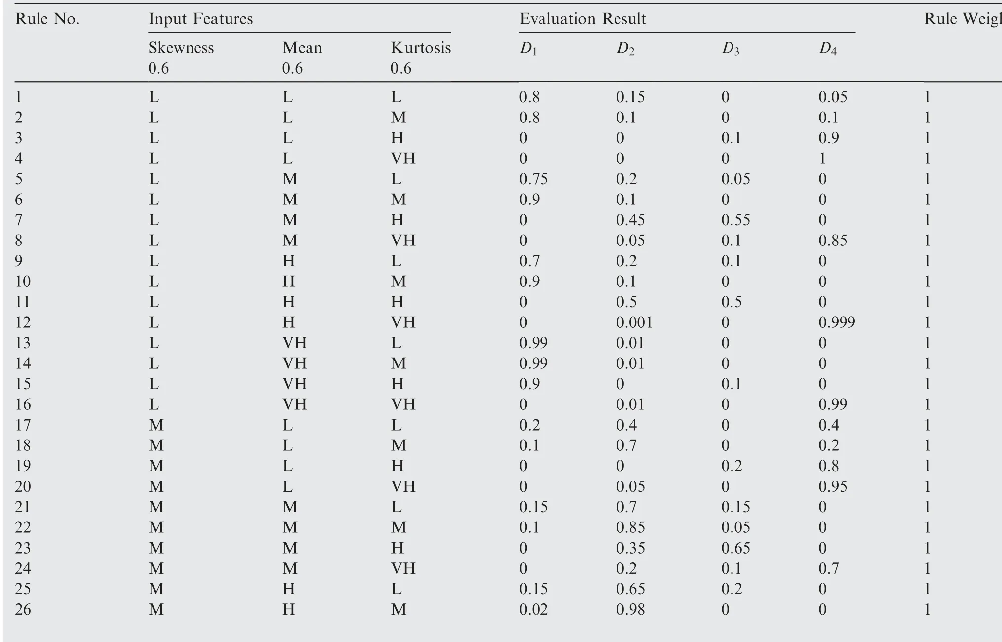
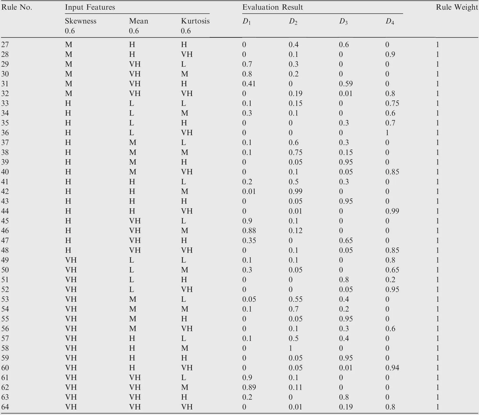
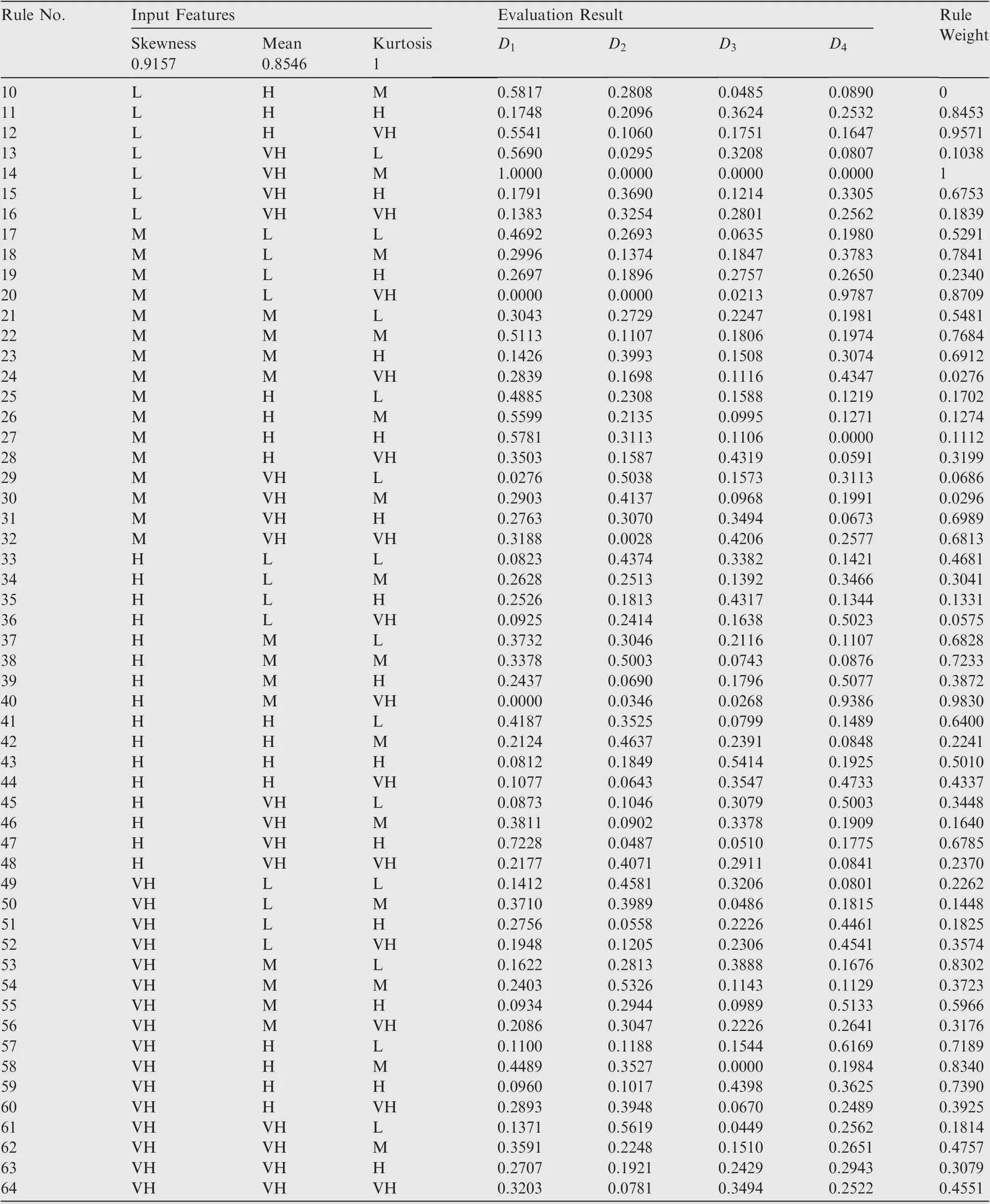
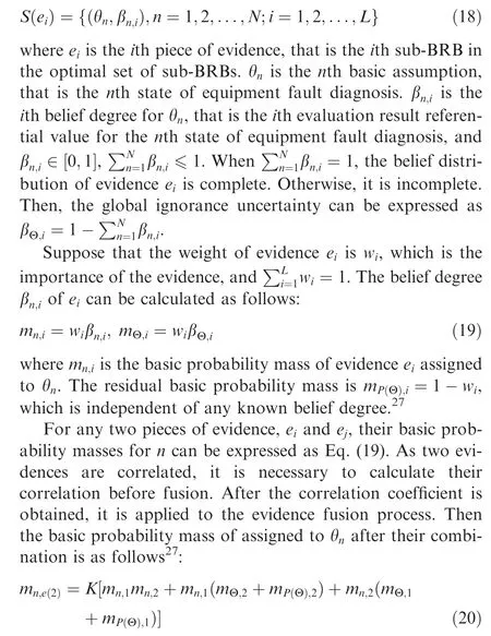
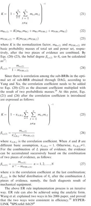
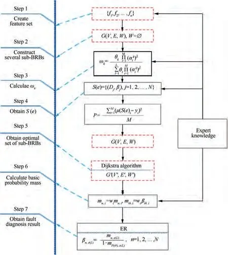
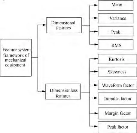
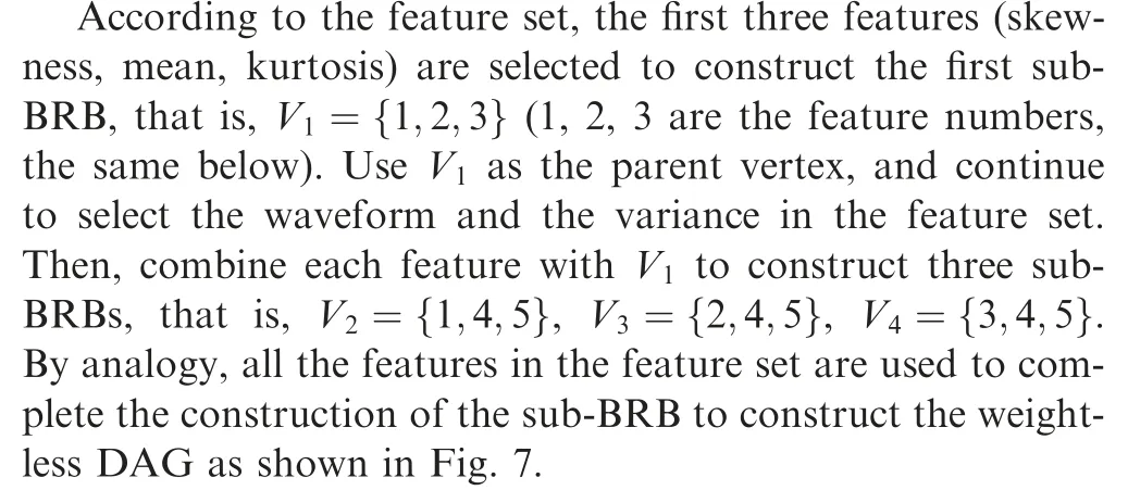
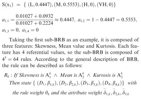
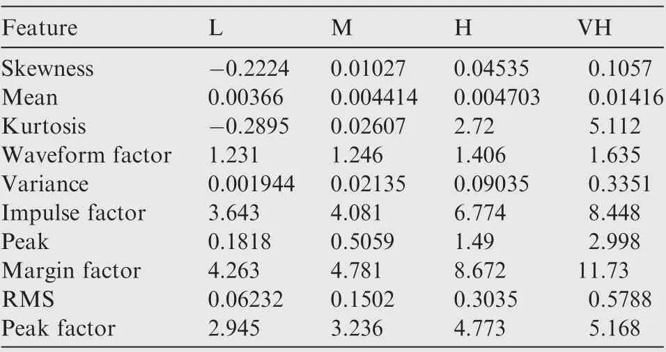
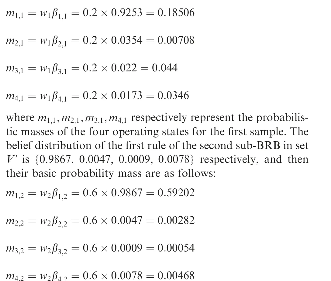
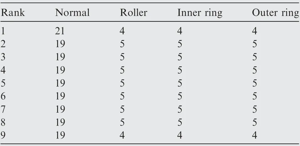
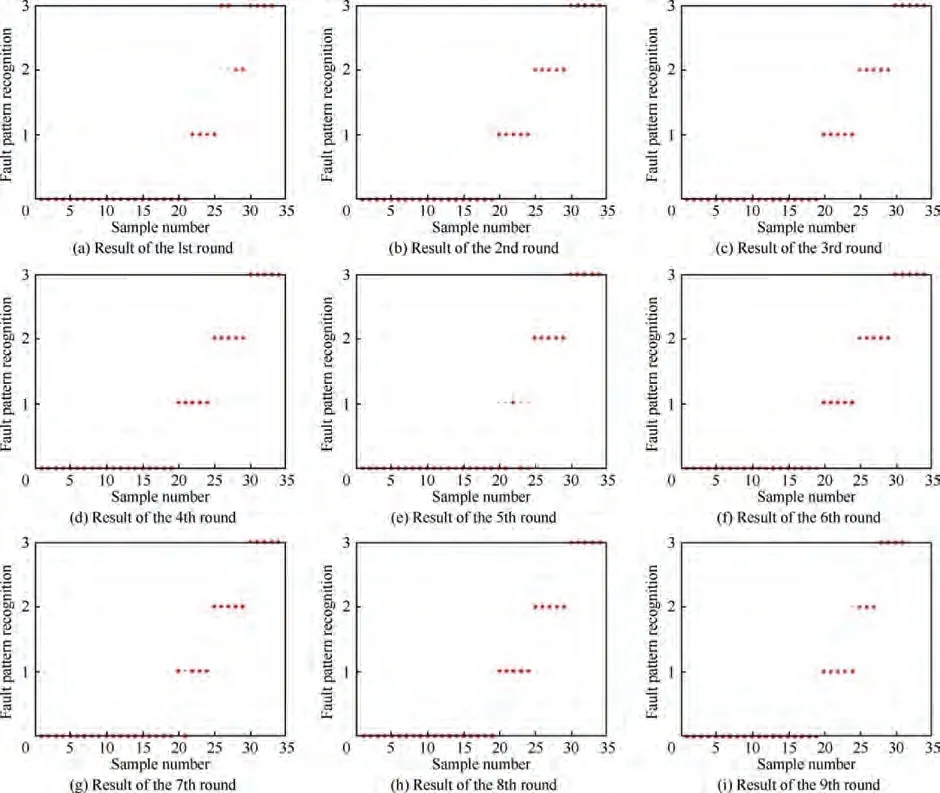
As shown in Table 5 and Eq. (15), the weight of the arc from the source point 1 to the first child vertex 6 of vertex 3 is calculated, and M is updated. If P+P Follow the above processes, and continue to calculate the weight of the arc from the source point 1 to remainder vertexes, until the third child vertex 9 of vertex 4. It is shown as follows: Continue traversing the remaining 16 vertexes as described above.Finally,Gis the shortest path,and Vis the optimal set of sub-BRBs.The three vertexes in Vdenote three sub-BRBs,each of which is composed of three features, and the structureis simple and calculation accuracy is higher.At the same time,because the structure of each sub-BRB is independent,parallel computation can be carried out and the efficient of execution is higher. However, because they come from the DAG, they are correlated.So vertex 4 is related to source point 1,and vertex 9 is related to vertex 4. Table 2 The 1st update of matrix M. Table 3 The 2nd update of matrix M. Table 4 The 3rd update of matrix M. Table 5 The 4th update of matrix M. Table 6 The nth update of matrix M. Evidential Reasoning(ER)rule is developed based on the evaluation analysis model and evidence combination rules of D-S theory.It is used to deal with uncertain knowledge in multiple features decision-making problems with qualitative and quantitative information.By introducing the concept of evidence weight, it effectively overcomes ‘‘counter-intuition”problem that may arise in the process of evidence fusion.It is a generalization of traditional Bayesian reasoning and D-S theory. ER rule provides a reliable solution for decisionmaking and evaluation with multiple pieces of evidence. In the equipment fault diagnosis problem,it is assumed that the possible state is θ(n=1,2,...,N), which can constitute a state set, namely the Frame of Discernment. This is defined as Θ={θ,θ,...,θ} where θdenotes the basic assumption.P(Θ) is the power set of Θ, which can be expressed as: In the previous section,each sub-BRB in the optimal set of sub-BRBs can obtain referential value of each operation state by Eq. (7), namely the belief distribution of the basic assumptions. Therefore, the belief distribution of θcan be expressed as follows: Based on the C-BRB model, a fault diagnosis process can be developed, as shown in Fig. 5.The whole steps are as follows: Step 1. According to the established feature system, the monitoring data collected by sensors are processed to obtain the corresponding feature values, and then the feature set is created based on the expert knowledge. Step 2. Features are selected from the feature set, and several sub-BRBs are constructed as the vertexes of DAG to establish the weightless DAG. Step 3. According to the expert knowledge, the referential values and weights of the features are set.The input feature value is transformed into the belief distribution corresponding to the referential values by Eqs. (2)-(4). The activation weight of each rule in each sub-BRB is calculated by Eq.(5).Step 4. In each rule of each sub-BRB, the initial weight of the rule and the initial belief degree of each evaluation result are set based on the expert knowledge. Then, Eqs.(6) - (10) are used to calculate the MSE of each sub-BRB,which is essentially the weight on the arc to complete the construction of DAG. Step 5.Based on the Dijkstra algorithm,the shortest path is obtained from the DAG, and then the optimal set of sub-BRBs is obtained. Step 6. According to the expert knowledge, the weight of each sub-BRB in the optimal set of sub-BRBs is given.Eq. (20) is used to calculate the basic probability mass of the belief distribution of each sub-BRB. Step 7.Eqs.(25)-(27)are used to fuse the basic probability mass of each sub-BRB to obtain the result of the fault diagnosis result of the equipment. The initial parameters of each sub-BRB in C-BRB model are set by experts. Considering the limitation of the expert knowledge, these parameters cannot satisfy the needs of actual environment.Thus, the parallel optimization of parameters is necessary. The parameters of sub-BRB that need to be optimized include the following 4 parts: θdenotes the weight of the kth rule; δdenotes the weight of the ith feature; γdenotes the referential value of the ith feature to the jth evaluation result; βdenotes the initial belief degree of the jth evaluation result. Thus, the objective function that is used to optimize the parameters of sub-BRB is proposed and shown as follows: Fig. 5 Equipment fault diagnosis algorithm of C-BRB. To solve the optimization problem shown in Eq. (28), in this paper,the Projection Covariance Matrix Adaption Evolution Strategy(P-CMA-ES) is used as the parallel optimization algorithm. It can solve the nonlinear continuous optimization problem, suitable for parameter optimization under all the constraints of BRB model.In addition, because each sub-BRB on C-BRB model can be optimized in parallel,optimization efficiency will be greatly improved. In order to verify the effectiveness of the proposed method, a case of fault diagnosis for rolling bearing is carried out in this paper. As the most precise basic parts in mechanical equipment, rolling bearings are widely used in modern industry.Because of many features, small samples and a large number of uncertain information, fault diagnosis for rolling bearing has always been a challenge. (1) Problem formulation. The monitoring data for the rolling bearing in various situations come from a simulation test rig set up by the Electrical Engineering Laboratory of the Case Western Reserve University. The type of rolling bearing is SKF6205,and the sampling frequency is 12 kHz. Under the working condition (2) (motor load = 735.49875 W, approximate speed = 1772 r/mi n),the operation under normal and three faults of roller,inner ring and outer ring are simulated respectively.The diameter of the faulty point is 0.1778 mm. The number of samples corresponding to each case is shown in Table 7. 192 samples of data are taken from normal vibration signals, where 134 samples are used as the training set, and 58 samples are used as the testing set.From each of the three kinds of vibration signals, 48 samples of data are collected, where 34 samples are the training set, and 14 samples are the testing set. There are 2500 sampling points for each sample. Table 7 Experimental dataset. On the whole,the amount of experimental data is relatively big. However, because the sampling frequency is high, which leads to the fact that the sampling interval is short, the difference between sampling points is not obvious. Therefore, each sample needs to contain more sampling points for assuring that extracted features are effective. To sum up, with only 336 samples of data at present, the example satisfies the small sample requirement of BRB. (2) Establishment of feature system. During the operation of mechanical equipment, a large number of signals can be obtained,which contain a large amount of system information and can reflect the operation state of the equipment.However,it is difficult to judge the operation states directly by observing signals.Thus, it is necessary to extract some main features for conducting the fault diagnosis first.To fully reflect the states of mechanical equipment, and retain the interpretability of the features, this paper takes vibration signals as an example, and uses the signal processing technology to extract the features of vibration signals.In the operation of mechanical equipment, the most direct manifestation of the fault is the occurrence of abnormal vibration,and therefore, the selection of vibration signals for fault diagnosis is a more reasonable method. The feature system framework of mechanical equipment for vibration signals is shown in Fig. 6. As shown in Fig. 6, the mean value can reflect the general situation of vibration signal of mechanical equipment.The variance can be used to describe the fluctuation range of the signal and the intensity of the vibration.Peak value, pulse factor and margin factor are used to detect whether there is an impact indicator in the signal.These three features can reflect the sensitivity of mechanical equipment faults.In the early monitoring, their values are different. Because the change of Root Mean Square (RMS) is not obvious, it is not suitable for early fault diagnosis. But RMS has good stability and can be used in combination with the first three features.Skewness and kurtosis are similar, which are used to describe the distribution shape of the signal.Skewness reflects the change through symmetry while kurtosis reflects the change through height, which can indicate whether the vibration data distribution of mechanical equipment is reasonable.The waveform factor is the ratio of root mean square to mean value, which can be used to judge the fault type.The peak factor is the ratio of the peak to the effective value,which usually increases slightly at the beginning of the fault, and decreases with the deterioration of the fault. According to Table 7 and Fig. 6, vibration signal features are extracted. Since it is difficult to distinguish the four possible cases of rolling bearings during the operation, all four dimensional features and six dimensionless features in the feature system are used to construct the feature set. After that, the dimensional features and dimensionless features are sorted in the order of intersection, so as to ensure that the two features are applied in each subsequent sub-BRB. The feature set is as follows: {Skewness, Mean, Kurtosis, Waveform factor, Variance,Impulse factor,Peak,Margin factor,RMS,Peak factor}. Fig. 6 Feature system framework of mechanical equipment for vibration signals. It should be noted that it is reasonable to select three features for each sub-BRB. At this time, the number of rules in each sub-BRB is fewer, which is easier to construct. Also,the number of vertexes of DAG is relatively few. Table 8 lists the influence on the number of sub-BRB rules and DAG vertexes. According to the four operation cases of rolling bearing,four different referential levels are set for input feature value,which are Low(L), Medium(M), High(H) and Very High(VH)respectively. The referential value is quantified as shown in Table 9,which is given by experts.With the gradual increase of each attribute value,the vibration of rolling bearing gradually becomes stronger, and the possibility of failure also increases. According to Eqs. (2)-(4), the belief distribution of input eigenvalues is calculated. For example, the first rule of the sub-BRB, that the Skewness is x=-0.0932, is transformed into the belief distribution: Fig. 7 Weightless DAG. Table 8 Influence of feature number on rule number and vertex number. Table 9 Quantitative table of feature referential value. For the three features in the kth rule, Mean is dimensional feature which is sensitive to the fault and will decrease with the occurrence of fault.It could identify whether there is the fault,but could not identify the type of the fault.Skewness and Kurtosis are dimensionless features which have strong antiinterference ability and small variations under normal conditions. When the fault occurs, Skewness gets bigger, and especially when the inner ring fault occurs,there are the maximum changes. Kurtosis changes only when the inner ring fault or outer ring fault occurs. According to the above analysis of three features, the initial value of each parameter in the kth rule is set, as shown in Table A1 of Appendix A. In the initial state, the 64 rules are considered equally important, so the weight of the rules is set to 1. The weight of Skewness, Mean and Kurtosis are all set to 0.6. The P-CMA-ES optimization algorithm is used for parameter optimization, the population size is set as 40 and the generation number is 300.The parameter values of the first BRB after optimization are shown in Table A2 of Appendix A. Based on the optimized parameters and the data from the training set, the belief distribution and MSE of this sub-BRB can be obtained by Eqs. (7)-(10). By analogy, the belief distribution and MSE of each sub-BRB can be obtained. On an arc, the MSE of the end point sub-BRB is used as the weight of the arc. Thus, the whole DAG is constructed. As shown in Table B1 of Appendix B,each arc in the DAG and its weights on the arc are displayed as a matrix, each weighted in 10units. According to Fig.7 and the weight of each arc in set W,the Dijkstra algorithm is used to obtain the path with the smallest sum of weights from the source point to the lowest vertex:shortest path, where vertexes construct the optimal set of sub-BRBs,namely,V={1,3,6,12,21},E={<1,3>,<3,6>,<6,12>,<12,21>},W={0.0048,0.005,0.0042,0.0047}. The MSE of the five sub-BRBs in set V’are{0.0065,0.0048,0.005, 0.0042, 0.0047} respectively. The smaller the value is,the higher the accuracy will be. Based on this criterion, the higher the accuracy is, the larger the weight will be. We set the weights of five sub-BRBs to be 0.2, 0.6, 0.4, 1 and 0.8 respectively. Eq. (19) is used to calculate the basic probability mass of the belief distribution of each rule in each sub-BRB.The belief distribution of the first rule of the first sub-BRB(source point 1) in set V’ is {0.9253, 0.0354, 0.022, 0.0173}respectively, and then their basic probability mass are as follows: where m,m,m,mrespectively represent the probabilistic masses of the four operating states for the first sample.According to the above process, the probability mass of samples in the source point 1 and the 3rd vertex can be obtained. Then the correlation coefficient of the source point 1 and the 3rd vertex is calculated.Jiang proposed a method to calculate the correlation coefficient in 2018.Compared with the traditional Pearson correlation coefficient, this method has stronger processing ability for discrete data, and is suitable for current case. The equations are as follows: where r(m,m) is the correlation coefficient of two evidences; mand mare the probability mass of samples; Aand Aare the focal elements of mass, namely, the basic assumption in the frame of discernment; N is the number of basic assumptions. In this case,there are four operation states of rolling bearings, and therefore, N=4. By Eq. (29) and Eq.(30), the correlation coefficient of the basic probability mass fusion of the first sample in the source point 1 and the 3rd vertex is calculated, that is, r(m,m)=0.99916. The larger the correlation coefficient is, the higher the correlation between the two data is.Therefore,there is a high correlation for the basic probability quality of the first sample in the source point 1 and the 3rd vertex. According to the above process,the correlation coefficient of probability mass of each sample is calculated in the source point 1 and the 3rd vertex,and there are 336 in total. Among them, the correlation coefficients of samples 1-10, 201-210, 251-260, and 301-310 are shown in Table 10. We can see from Table 10 that there is a strong correlation between source point 1 and the 3rd vertex. The correlation coefficient is substituted into Eqs. (25) and (26) to carry out the fusion calculation of source point 1 and vertex 3, and the fusion result of two evidences is obtained. In this way, the fusion result of source point 1 and vertex 3, 6, 12, 21 can be finally obtained, that is, the result of C-BRB model aimed at the fault diagnosis of rolling bearing, as shown in Fig. 8. It can be seen from Fig. 8 that one Dis mistaken for D,five Dare mistaken for D, one Dis mistaken for D, and one Dis mistaken for D. Table 11 clearly reflects the performance of C-BRB in fault diagnosis of rolling bearings. TP, FN, and FP are the number of true positive,false negative and false positive results,respectively. The True Positive Rate (TPR) of C-BRB is more than 95%. With the exception of D, the Positive Predictive Value(PPV) of C-BRB is over 95%. Fig. 8 and Table 11 show thatC-BRB can obtain satisfactory results in fault diagnosis of rolling bearings. Table 10 Correlation coefficients of partial samples in source point 1 and 3rd vertex. Fig. 8 Result of fault diagnosis of C-BRB. Table 11 Fault diagnosis performance of C-BRB. Table 12 Comparison with non-optimized C-BRB and traditional BRB. According to Table 12, the detailed comparison of performance is given. Except that the PPV of Dis lower than the Initial C-BRB, the performance of C-BRB is higher than the Initial C-BRB, which illustrates the importance of the optimization for the C-BRB. The TPR and PPV of C-BRB are higher than the traditional BRB. In the case of ten features and four referential values for each feature, the traditionalBRB requires 4=1048576 rules to be built. This makes the expert knowledge not be used, and the parameters of rules can only be set randomly. Thus, the TPR and PPV of CBRB are higher than those of the traditional BRB. From this aspect, the performance of C-BRB is better than that of the initial C-BRB and the traditional BRB, which also verifies the effectiveness of the proposed method. Table 13 Cross validation dataset. (1) Cross validation. To further verify the reliability of the proposed method, 9 rounds of cross validation are designed in this paper. By dividing the monitoring data into 9 groups, each group includes normal and three faults of roller, inner ring and outer ring respectively.There are 2500 sample points for each set of data in each group, as shown in Table 13. When each round of cross validation is performed, one group is selected from 9 groups as the testing set, and other groups are used as the training set.By the optimal parameters of C-BRB, the results of 9 rounds of cross validation are shown in Fig. 9. It can be seen from Fig. 9 that the 1st, 5th and 9th rounds have some diagnostic errors, while the 2nd, 3rd, 4th, 6th, 7th and 8th rounds do not have errors.The average TPR and PPV of each round of cross validation can be shown in Table 14. Fig. 9 Results of 9 rounds of cross validation. Table 14 Performance of each round of cross validation. Fig. 10 Results of fault diagnosis of FS-BRB. It can be seen from Table 13 that in the above 9 rounds of cross validation, only the PPV of the 5th round is lower. In addition, the results of other rounds stay at a high level with small fluctuations. Therefore, cross validation shows that the proposed method is reliable. (2) Comparison with FS-BRB(Features Selection BRB).In order to further illustrate the effectiveness of C-BRB,the model is compared with FS-BRB. The features are selected by the correlation between the observation data of features and the fault diagnosis output, and the 7th and the 9th features (Peak and RMS) are used as the inputs of the FS-BRB. The training data and the optimization algorithm of the FS-BRB are the same as those of the C-BRB. The model output is shown in Fig. 10. It can be seen from Fig. 10 that one Dis mistaken for Dand twelve Dare mistaken for D.The performance comparison between FS-BRB and C-BRB is shown in Table 15. Table 15 Performance comparison between C-BRB and FSBRB. It can be seen from Table 15 that C-BRB has stronger fault diagnosis ability than FS-BRB when it comes to fault diagnosis of rolling bearings.This is because FS-BRB selects features during the fault diagnosis, which leads to information loss. In the case of small sample, there is less information after selection, which affects its diagnostic accuracy. (3) Comparison with BP. To further illustrate the effectiveness of C-BRB, a comparison with BP neural network model is studied. The fault diagnosis result of the BP model for the rolling bearing is shown in Fig. 11. It can be seen from Fig.11 that five Dare mistaken for D,two Dare mistaken for D,and four Dare mistaken for D.The performance comparison between BP and C-BRB is shown in Table 16. It can be seen from Table 16 that C-BRB has stronger fault diagnosis ability than BP when it comes to fault diagnosis of rolling bearings.When using BP for fault diagnosis,it is necessary to use big data for training, which leads to insufficient model training when the data is small, affecting the diagnosis results. When using the method proposed in this paper, due to the use of the expert knowledge for model construction and parameter setting, fault diagnosis can be carried out in the case of small data, and better results are obtained. Therefore, the above results show that the proposed method is effective. Fig. 11 Results of fault diagnosis of BP. Table 16 Performance comparison between BP and C-BRB. In this paper, a C-BRB model for fault diagnosis of mechanical equipment is proposed to solve the problem of small sample and make the description of uncertain information. The numerical simulation experiment and comparative study of rolling bearing show that the proposed method can not only disperse multiple features into several optimal sub-BRBs, but also fuse the optimal sub-BRBs to achieve a comprehensive fault diagnosis of the equipment. The main contributions of this paper include two aspects.First, the C-BRB model is proposed to use multiple features,in which several sub-BRBs containing only a few features are created and used to generate a DAG.Afterwards,the Dijkstra algorithm is used to obtain the optimal set of sub-BRBs where the feature integrity and accuracy and execution efficiency of BRB are taken into account. The C-BRB model reduces the rules number of BRB and avoids the rules of BRB to combine explosion. Second, the ER rule with correlation coefficient is employed to combine all the sub-BRBs in the optimal set to obtain the fault diagnosis result of the equipment,which meets the requirement of multiple features application. Although the proposed fault diagnosis method based on DAG and BRB with multiple features cases is validated to be effective,its ability in dealing with more practical and complex problems needs to be examined.In addition,the extracted features are affected by many environmental factors. Therefore, it is necessary to further study the robustness of the model in the future when the monitoring data are disturbed. The authors declare that they have no known competing financial interests or personal relationships that could have appeared to influence the work reported in this paper. This work was supported by the Natural Science Foundation of China (Nos. 61773388, 61751304, 61833016, 61702142,U1811264 and 61966009), the Shaanxi Outstanding Youth Science Foundation, China (No. 2020JC-34), the Key Research and Development Plan of Hainan, China (No.ZDYF2019007), China Postdoctoral Science Foundation(No.2020M673668),and Guangxi Key Laboratory of Trusted Software, China (No. KX202050). Appendix A. First sub-BRB of C-BRB Table A1 Initial parameters of the first sub-BRB. Table A1 (continued) Table A2 Optimized parameters of the first sub-BRB. Table A2 (continued) Appendix B. The weight of arcs on the DAG Table B1 The matrix of weight of arcs.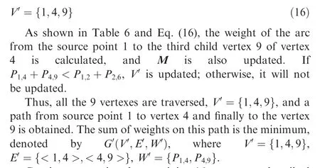


3.3. Fusion process based on the ER rule

4. Fault diagnosis process based on C-BRB
4.1. Construction of fault diagnosis model
4.2. Parallel optimization of fault diagnosis model

5. Case study
5.1. Experimental preparation

5.2. Construction of initial C-BRB for fault diagnosis of rolling bearing

5.3. Training and testing of C-BRB fault diagnosis model


5.4. Comparative study


6. Conclusions
