A new target tracking filter based on deep learning

Yaqi CUI, You HE, Tiantian TANG, Yu LIU

Naval Aviation University, Yantai 264001, China

KEYWORDS Attention mechanism;Feedforward neural network;Interactive multiple model;Recurrent neural network;Tracking filter

Abstract At present,current filters can basically solve the filtering problem in target tracking,but there are still many problems such as too many filtering variants, too many filtering forms, loosely coupled with the target motion model,and so on.To solve the above problems,we carry out crossapplication research of artificial intelligence theory and methods in the field of tracking filters. We firstly analyze the computation graphs of typical α-β and Kalman. Through analysis, it is concluded that α-β and Kalman have the same computation structures analogous to a typical recurrent neural network and can be considered as a kind of recurrent neural network with constrained weights.Then,given this and considering that a recurrent neural network has the recognition capability for target motion patterns, a new filter is developed in a unified neural network architecture and specifically constructed using feedforward neural network,recurrent neural network,and attention mechanism.And the unified tracking filter proposed in this paper can generate three aspects of unity:a unified target motion model,an adaptive filter method,and an overall track filtering framework. Finally, Simulation results show that the proposed filter is effective and useful, of which the overall performance is superior to those of compared filters.

1. Introduction

Tracking filter is the core part of target tracking.Its main function is to estimate target motion states accurately and in realtime from noisy radar measurements.Its performance has a decision on the final target tracking effect. Before deep learning was brought up, researchers usually made an effort from two aspects to achieve better performance:one was to establish a motion model in consistent with a target’s actual movement;the other was to adopt a matched filter.In the aspect of target motion models, there are mainly two kinds: single-mode and multi-mode.Typical single-mode models include Constant Velocity (CV) model, Constant Acceleration (CA) model,Constant Turning (CT) model, Singer model, Jerk model,and current statistical model. Because one single-mode model can only cover one moving pattern and a target’s actual movement is time-varying, the performance of single-mode models is unstable.For example,a CV model can guarantee a tracking effect on targets moving at a constant speed. Nevertheless, if the actual moving pattern is CA or CT, or is more likely CV at the beginning but changes to CA or CT later, the performance will become worse, which will lead to abnormal problems such as tracking errors and losses. On the contrary, a multi-mode motion model is essentially a comprehensive integrated framework, which improves the overall performance of a tracking filter by integrating multiple single-mode motion models at the expense of the optimal performance.Interactive Multi-Model (IMM) is a typical model. Although a multi-mode motion model can enhance the ability to cover different kinds of motion patterns by integration, existing methods can just integrate a very limited number of motion models due to competition and pollution effect among the models. Therefore, the expression ability of existing multimode motion models is still very limited,and the actual motion pattern of a target still cannot be fully described accurately.

In the aspect of filters, current methods can be classified into two groups: linear and nonlinear filters. Linear filters include α-β,Kalman,and so on,which can be used to solve the linear system filtering problem. Nonlinear filters include Extended Kalman Filter (EKF) derived by first-order linear approximation,Unscented Kalman Filter (UKF) derived by three-order linear approximation,Cubature Kalman Filter(CKF) with higher accuracy,and Particle Filter (PF) using random sampling approximationand Gaussian Mixture Probability Hypothesis Density (GM-PHD) to solve the multi-target filtering problem.At present, current filters can solve the filtering problem in target tracking,but there are still many problems such as too many filtering variants, too many filtering forms, loosely coupled with the target motion model,and so on.

Meanwhile, with the advancement of research on machine learning and deep neural network, it has become a new research direction to carry out cross-application research of artificial intelligence theory and methods in the field of tracking filters.Moreover,we denote filters not based on neural networks as for traditional filters. We can simply divide current research on tracking filtering based on neural networks into three categories. (A) Union style. This style unites neural networks and traditional filters without changing traditional filters to improve the ability to solve a problem. (B)Replacement style. This style replaces modules or estimates parameters in traditional filters without changing those frameworks to improve the filter performance.(C)Remodeling style.This style realizes the whole filtering function using neural networks,which completely breaks the frameworks and compositions of traditional filters.

For union style, related studies include Refs. [10-14]. Ref.[10]proposed an implementation of the generalized regression neural network to obtain location estimates of a single target moving in 2-D in wireless sensor networks, which were then further refined using Kalman.Refs.[11,12]predicted measurements for UKF during the signal outages of Global Navigation Satellite System (GNSS) using neural networks to improve the position and velocity precision of the integrated navigation system based on Inertial Navigation System (INS)and GNSS. Ref. [13] integrated Kalman in the middle of an encode-decode neural network to transform the nonlinear filtering problem in a space of low dimensions to the linear filtering problem in a space of high dimensions based on the kernel thought.

For replacement style,there have been a lot of studies.Ref.[15]adopted a simple neural network as the target moving model and used it to realize a one-step prediction of the target state in Kalman. Refs. [16,17] adopted Long Short-Term Memory (LSTM) as the target moving model and used it to realize a one-step prediction of the target state in Kalman by estimating the mean and covariance of predictions, which could partially solve the problems of weak expression and mismatching in traditional filters.Ref.[18]learned the consistency of the innovation sequence in Kalman using deep belief networks to automatically adjust the covariance of the process and measurement noises, which could partially solve the difficult problem of parameters adjustment in traditional filters.Ref. [19] estimated a prediction of the target state, the covariance of the process noise, and the covariance of the measurement noise respectively using three LSTMs. Ref. [20]adopted LSTM as the target moving model and used it to realize a one-step prediction of the target state in a PF. Ref. [21]implemented a one-step prediction for the single Gaussian state from a Gaussian mixture respectively using LSTM in GM-PHD. Ref. [22] implemented a one-step prediction for a whole Gaussian mixture using ConvLSTM in GM-PHD.

For remodeling style,there has been few research including Ref. [23] published in 2009. This paper showed that the filtering ability of one-dimensional Kalman could be realized by a recurrent neural network, of which the parameters are set according to the parameters of Kalman.Because deep learning has not yet been proposed in 2009, people’s understanding of neural networks and network learning was very limited.Hence, this paper only demonstrated that neural networks could realize Kalman, but didn’t consider using neural networks to further improve the performance of Kalman. In addition, the parameters of the neural network in this paper were all given directly without training, which was quite different from current implementation method of neural networks.

In general,a target tracking filter still lacks unity in the following three aspects at present:

(1) There is a lack of a unified filtering method that can adaptively match the track filtering problem, but the existing filters are only the specific filtering realization for different problems obtained by different thoughts.

(2) There is a lack of a unified framework to integrate motion models and filtering methods, but the existing implementations for the two parts are selected separately and connected sequentially.

(3) Though current research on track filtering based on neural networks solve problems of weak expression and mismatching, the corresponding filters are still in the framework of traditional filters, and we still do not get a unified framework.

To solve the above problems, we carry out crossapplication research of artificial intelligence theory and methods in the field of tracking filters according to the remodeling style.We firstly analyze the computation graphs of typical and Kalman. Through analysis, it is concluded that and Kalman have the same computation structures analogous to a typical recurrent neural network and can be considered as a kind of recurrent neural network with constrained weights. Then,given this and considering that a recurrent neural network has the recognition capability for target motion patterns, a unified tracking filter is proposed to generate three aspects of unity: a unified target motion model, an adaptive filter method, and an overall track filtering framework. Finally,the availability and effectiveness of the proposed method are verified by simulation experiments and contrastive analysis.

2. Computation graph analysis of typical filters

Firstly, the existing α-β and Kalman are analyzed and explored from the perspective of computation graph,the structure characteristics to guide developing a unified tracking filter.In the following, a computation graph would be constructed by nodes and directed edges between different nodes. Specifically,directed edges will be denoted with arrows and only used to represent data transferring from the node in the opposite direction of the arrow to the node in the direction of the arrow,aqua rectangular nodes will be used to represent inputs, lilac rectangular nodes to represent parameters,orange rectangular nodes to represent outputs, olive circle nodes to represent different computations including add, subtract, multiply, and complex functions, and black rectangular nodes to represent the special time delay. Meanwhile, to distinguish a neural network architecture graph from a computation graph, rounded rectangles will be used to represent different layers in the neural network, and the color usage in the neural network architecture graph is consistent with that of the computation graph. Specifically, the aqua rectangles with rounded corners will be used to represent the input layer, the orange rectangles to represent the output layer,and the olive rectangles to represent the hidden layer.

2.1. Computation graph analysis of the α-β filter

As a linear and fixed-gain filter, α-β is the steady-state solution of Kalman, and its performance is the same as that of a steady-state Kalman.Because of its simple form,the computation graph of α-β is analyzed at the beginning.

The α-β formula can be simply expressed as follows:

where X is the target state vector, z is the radar measurement vector, F is the state transform matrix, H is the measurement matrix, k is previous moment, k+1 is current moment, X（k|k） is the state estimation vector at time k,X（k+1|k） is a one-step prediction for the target state at time k, X（k+1|k+1） is the state estimation vector at time k+1, K is the fixed gain, and T is the time interval between current and previous moments. According to specific questions, X, F, H, and K can have different vector settings.Moreover, for a one-dimensional constant-velocity motion model,atypicalvectorsettingaboutKis K=diag（［α， β/T］）.

From the point of algorithm integrity,the initialization step should be included here. However, the initialization step belongs to the additional pretreatment process in the implementation of a filter and is a universal step for different filters in essence. Hence, considering independence and universality,the initialization step is not included in the α-β filter and the following Kalman filter.

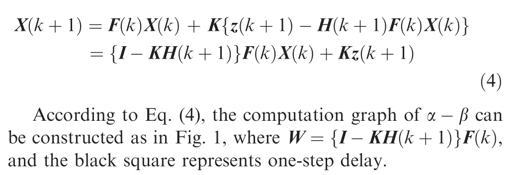
By substituting Eqs.(1)and(3)into Eq.(2)and expanding,the direct relationship between X（k+1|k+1） and X（k|k） can be obtained as follows:

The Fig. 1 shows that in addition to typical computation operations such as addition and multiplication in the filter,there is a special delay feedback structure, which is shown as the bold connection lines. Combined with Eq. (4), it can be seen that the delayed feedback structure can integrate past and present information,and has the function of smooth filtering, which is the core structure of α-β.

2.2. Computation graph analysis of Kalman filter

Kalman is a widely used, studied, and developed filter, which occupies a dominant position in the field of tracking filter. In comparison with α-β, the outstanding characteristic in Kalman is that the gain K is calculated in real time. The gain in Kalman represents the relative quality estimation of present measurement and can be dynamically calculated based on both past and present measurements. The calculation equations for the gain are as follows:

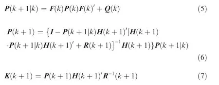
where Q is the covariance of the process noise,P is the covariance of the state vector estimation, and R is the covariance of the measurement noise.

Because Eqs. (5)-(7) contain an inverse operation of the matrix,it is difficult to express them directly using a computation graph. However, from the point of view of input-output information flow, the calculation equations for the gain can be synthesized and simplified as below.

Firstly, the following equation can be obtained through simplifying Eqs. (5) and (6):

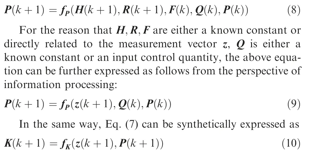
According to Eqs. (9) and (10), the computation graph of the gain in Kalman can be constructed as in Fig. 2. Furthermore, combined with Fig. 1, the computation graph of the whole Kalman can be obtained as shown in Fig. 3.

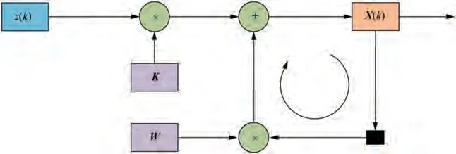
Fig. 1 α-β filter computation graph.

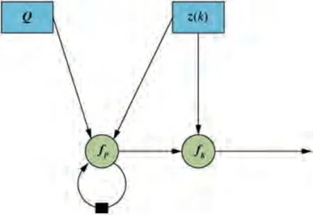
Fig. 2 Computation graph of the gain in Kalman.

It can be seen from the Fig.3 that the computation graph of the whole Kalman includes linear operations such as addition and multiplication,and nonlinear operations such as fand f,as well as two delayed feedback structures, which are the core units of Kalman, one to calculate the filter gain and the other to smooth the filter.

Therefore, by constructing and analyzing the computation structures of typical filters like α-β and Kalman, as well as making analogies to other filters,it can be found that a delayed feedback structure is the key structure to realize filtering.Hence, by designing a more general delayed feedback structure, a filter in a more unified form and with a better performance can be realized.

3. A unified model

From the point of view of computation graph, typical filters include linear operations,such as addition,subtraction,multiplication,division,nonlinear operations,and delayed feedback structures, which can all be realized by a neural network.Therefore, according to the structural characteristics of existing filters and based on the functional characteristics of various neural networks, a Unified Tracking Filter (UTF) is derived.

3.1. Typical neural network structure

A target tracking filter corresponds to time series processing problems in neural networks, and relevant neural network structures include feedforward neural network structures,recurrent neural network structures, and attention mechanisms.Their functional characteristics are described respectively as follows.

(1)A feedforward neural network structureis shown in Fig. 4,which includes an input layer, one or more hidden layers, an output layer, interlayer connection weights, and omitted bias terms. In Fig. 4 and Fig. 5, U, V, and W are defined as the connection weights and fas the activation function.In addition,the activation function fis pre-set when designing the neural network and can be None function, Sigmoid function, Tanh function, ReLu function, Softplus function, etc.U, V, and W are matrices or tensors which need to be solved by training the neural network. Therefore, the calculation function, for example, between the input layer and the first hidden layer,is h=f（Uz+b）,and the bias term b is omitted.

According to the universal approximation theorem, the feedforward neural network can fit an arbitrary complexity function in any precision only using a single hidden layer with a few neural units.

Fig. 3 Computation graph of whole Kalman.

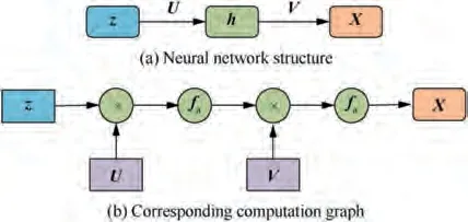
Fig. 4 Feedforward neural network.

(2) A recurrent neural network structureis shown in Fig. 5. Based on the feedforward neural network, a delayed feedback line is added to strengthen the time connection among the hidden layers at different times and transmit the neural unit value at previous moments to the current neural unit. Consequently, the recurrent neural network structure has the ability of memory and can deal with time series problems with context. Basic and typical structures of recurrent neural networks include simple recurrent neural network,LSTM recurrent neural network,and Gated Recurrent Unit(GRU).

(3)The attention mechanismin neural networks comes from the human visual attention mechanism, which can dynamically adjust the weights of input information according to different task scenes and focus more attention on the highvalue and useful part of the input information to improve the effectiveness and accuracy of information processing.A typical attention mechanism is shown in Fig. 6. The actual computation about attention weights can be abstractly described as a mapping of a query to a series of key-value pairs. It mainly includes three calculation steps as shown in Eq. (11), which are similarity calculation, normalization, and weighted sum,respectively.

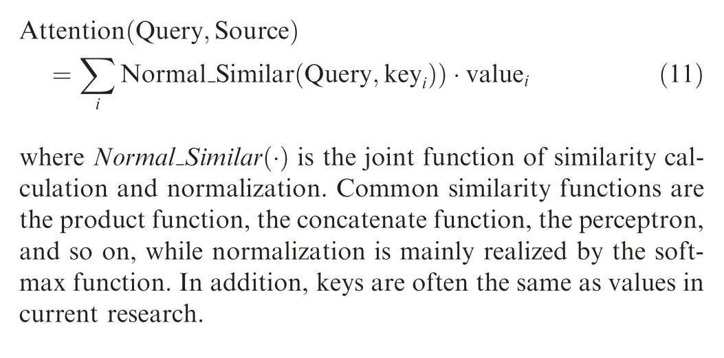
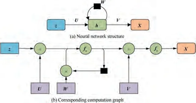
Fig. 5 Recurrent neural network.

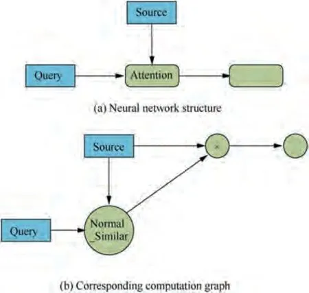
Fig. 6 Attention mechanism.

By contrasting the computational structures of typical filters with those of classical neural networks, it can be found that all the typical filters can be completely realized through neural network structures.

(1) By comparing Fig. 1 with Fig. 5, it can be concluded that α-β can be directly expressed using the structure of a recurrent neural network as shown in Fig. 7. The input layer consists of a measurement vector, the hidden layer consists of a state vector,and the output layer directly outputs the hidden layer.

(2) By comparing Fig. 3 with Fig. 5 and Fig. 6, it can be concluded that Kalman can also be expressed using a multilayer recurrent neural network with an attention mechanism as shown in Fig. 8. The dashed line in the figure indicates the information connection existing in the actual Kalman filter but omitted in the neural network implementation.Due to that the neural network emphasizes the perceptual structure and information flows,it should approximate the specific equation and should not be restricted to the specific equation expression. Out of the above consideration, it is reasonable to omit the dashed line because that K information has flowed into X through the attention connection.

Fig. 7 Neural network structure of α-β filter.

Through the above comprehensive comparison and analysis, it can be concluded that the nonlinear operation in a filter can be expressed as a feedforward neural network structure,the delayed feedback as a constrained recurrent neural network structure, and the filter gain as an attention mechanism.Therefore, a unified tracking filter can be constructed using basic neural network modules,such as feedforward neural network, recurrent neural network, and attention mechanism.

3.2. Unified tracking filter

For the simple α-β filter, the basic principle is to use historical measurements to constrain and decrease the fluctuation of current measurement through operations of the delayed feedback and the weighted average. In addition, the final effect of the α-β filter is to smooth the fluctuant measurements and obtain stable estimations of the target state. Hence,according to the function and effect of the α-β filter,the corresponding neural network as shown in Fig.7 is called smooth network and is composed of feedforward and recurrent structures.For the complex Kalman filter,the basic principle is the same as that of the α-β filter, but the gain in the Kalman filter that is calculated in real time using the quality information of current and historical measurements is different from the gain in the α-β filter that is set as a constant in advance.Hence, compared with the α-β filter, an additional neural network is needed to realize the calculation for the gain,which is called evaluation network according to the calculation process that utilizes the quality information.According to the neural network structure of Kalman shown in Fig. 8, the evaluation network is mainly constructed by feedforward structures, recurrent structures, and an attention mechanism.Meanwhile, an additional attention mechanism is used to transfer the gain information from the evaluation network to the smooth network and integrate the two network parts closely.

Hence, by making an analogy about computation structures between classical filtering methods and typical neural networks, a unified tracking filter is derived following the computation graph of typical filters and by taking a multilayer feedforward neural network and a recurrent neural network as the main units and introducing an attention mechanism additionally.As shown in Fig.9,the unified tracking filter includes three parts, i.e., an evaluation network, an attention mechanism, and a smooth network. The evaluation network, which realizes an evaluation of measurement information, receives external control and measurement information and outputs the related information of the filter gain by synthesizing past and present information. The attention mechanism couples gain-related information from the evaluation network with measurement information to select measurement information.The smooth network synthesizes the past state and new input information to obtain an estimation of the current state ultimately.

Meanwhile, Refs. [16-17,19-22] have proven that a recurrent neural network added with a multilayer feedforward network can extract and identify many different motion patterns mixed in tracking data. Considering that, the unified tracking filter not only possesses filtering ability but also has the ability of extracting and recognizing different motion patterns.Hence, it can be deduced that the unified tracking filter has the whole ability of filtering for targets moving in any motion pattern.

About Fig. 9 and Fig. 10, there is something that needs to be stated. In a neural network, there are two ways to describe the algorithm:one is to adopt multiple functions as in the traditional α-β and Kalman methods,and the other is to adopt the block diagram which is commonly used in neural networks for effectively representing the relationship between network layers. Moreover, the two ways of representation method are equivalent, and behind the block diagram are complicated functions. Because the key point in this paper is to develop a new filter based on deep learning from the point of computation graph and computation structure using feed-forward neural networks, recurrent neural networks, and attention mechanisms which are all known, the functional block diagram is adopted to describe the unified tracking filter as shown in Fig. 9 and Fig. 10.

3.3. Simple implementation of the unified tracking filter

The above section just gives a unified model,not a concrete filter method.To verify the performance of the unified model by comparison with existing filters such as α-β, Kalman, and LSTM-Kalman, it is necessary to design and construct a concrete filter based on the unified tracking filter,which is referred to as the Unified Filtering Neural Network (UFNN) hereinafter. In the process of designing and implementing the unified filtering neural network,the following key points would be considered.

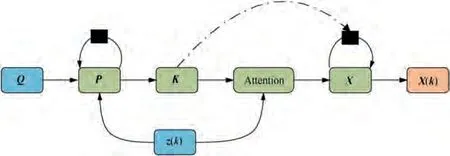
Fig. 8 Neural network structure of Kalman.

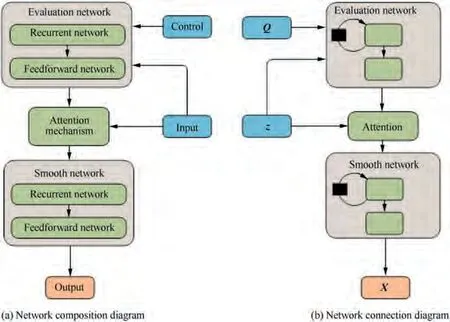
Fig. 9 Unified tracking filter.

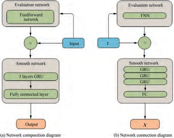
Fig. 10 Unified filtering neural network.

(1) In experimental verification, the main purpose is to verify the feasibility of the unified tracking filter.Given the capability and application scope of existing filters, the complexity and size of the unified filtering neural network should not be excessively big.

(2) In training and learning for the neural network,the size of training data must match the size of the neural network.In the case of few training data,it is not appropriate to use a big neural network with too many parameters, which is difficult to train.

(3) In an actual filtering process for target tracking,the control information is usually not input,and Q is known as a constant.Hence,in specific implementation of the unified tracking filter, the input Q can be omitted, and the information carried by the constant Q can be represented by the bias term in the neural network;

(4) Because the recurrent neural network already contains a few layers of the feedforward neural network,the subsequent multilayer feedforward network can be simplified to a fully connected layer.

In the light of the above consideration, a unified filtering neural network is derived from the unified tracking filter as shown in Fig. 10. Specifically, the evaluation network is realized using the feedforward networkwith a single hidden layer. According to the first key point, the attention mechanismis implemented by a simple weighted method, which is the simplest attention mechanism. The front part of the smooth network consists of three gated recurrent unitswith a descending number of cells as shown in Fig.11,where σ and Tanh are respectively the sigmoid activation function and the hyperbolic tangent activation function, and the hidden states H（k ） and H（k+1） are the states of the hidden layer at different time steps. Meanwhile, the latter part of the smooth network is just a fully connected layer.In addition, the number of neural units in every layer of the unified filtering neural network can be specifically determined and adjusted according to the actual training evaluation.

4. Experimental validation

Because the benchmark data set for target tracking in radars has not been established, it is hard to use real data to test the proposed method. Hence, the performance of the unified tracking filter is analyzed and evaluated using experimental simulation and by comparison with typical filters. In the comparative experiment, the existing filters used for comparison include α-β, Kalman, and LSTM-Kalman.The whole experiment is based on Keras and Tensorflow library and implemented by Python language, and detailed configurations about this experiment are as follows: Ubuntu 16.04, 16 GB RAM, Xeon E5-1620 v4 3.5 GHz, and no GPU.

4.1. Simulation settings

The simulation scenario assumes that a two-coordinate radar tracks a single target, filters the corresponding measurements,and finally estimates the target state.In accordance with traditional simulation practice, the two-coordinate radar is assumed to be determined with fixed measurement noises,namely the fixed ranging and direction-finding errors, and the target is in various states with different initial positions,speeds,courses,and movement modes during one-time simulation. Specifically, the radar is assumed to measure the target distance and azimuth at a 1 s period with zero mean Gaussian white noise,of which the range standard deviation is 50 m and the azimuth one is 0.01745 radian (1°). Moreover, the radar measurement for the target range and azimuth in the polar coordinate system would be directly transformed to the rectangular coordinate system through modified transformation equations between the polar and rectangular coordinate systems. In the target part of the simulation setting, the target is assumed to motion starting from a random initial state and in a single-mode pattern or a multi-mode hybrid pattern based on CV, CA, and CT which are modeled by setting the state transform matrix in Eq. (1) as shown in Eq. (12), and the entire target movement lasts for 20 s. The initial state of the target includes the initial position p, the initial velocity v, the initial acceleration a, and the angular turning rate w,and all comply with uniform distribution, of which the distribution range is shown in Eq. (13).

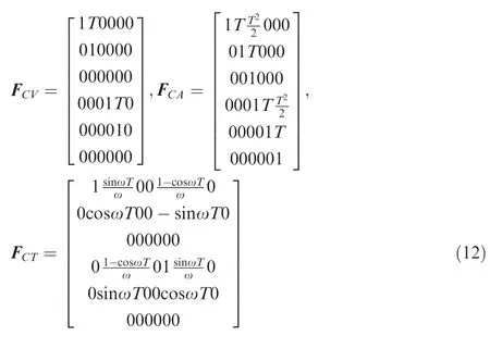
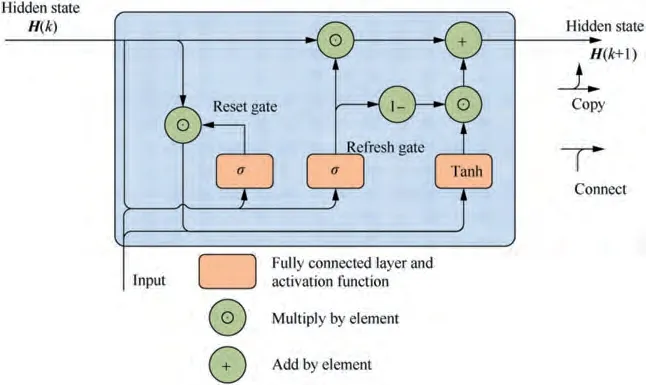
Fig. 11 Gated Recurrent Units (GRU).

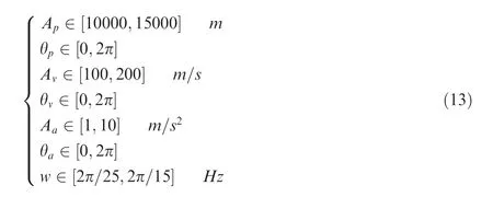
where F， F， Fare the state transform matrices for CV,CA,and CT,respectively,T is the sampling interval and set to 1 s,ω is the turning speed in CT,A indicates the amplitude distribution, and θ indicates the angle distribution.

Because the target position measurement is nonstationary and cannot be directly input into neural networks, it is necessary to preprocess and transform nonstationary data to stationary ones for filtering estimation using the unified filtering neural network. As for targets velocity, considering that various scopes of these can be determined in advance and the amplitude of the variation is relatively small, they can be assumed to be approximately stationary. Therefore, a final tracking filter network is constructed as shown in Fig. 12.Firstly, based on one unified filtering neural network, a velocity estimation of the target can be obtained by differential treatments for the original measurement sequences from a radar. Then, according to the newly estimated velocity, a prediction for the target position can be obtained.Further,based on the other unified filtering neural network, the residual errors between the actual radar measurement of the target position and the predicted position can be calculated and estimated. At last, a position estimation of the target can be obtained by adding up the estimation of residual errors and the predicted position.Therefore,to track and filter the target,it is necessary to train and optimize the two unified filtering neural networks respectively, which are termed as the velocity network and the position network next.

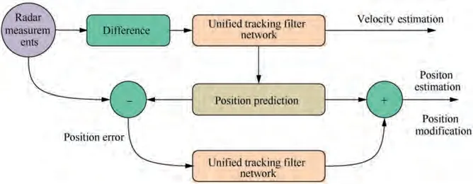
Fig. 12 Target tracking and filtering using two unified filtering neural networks.

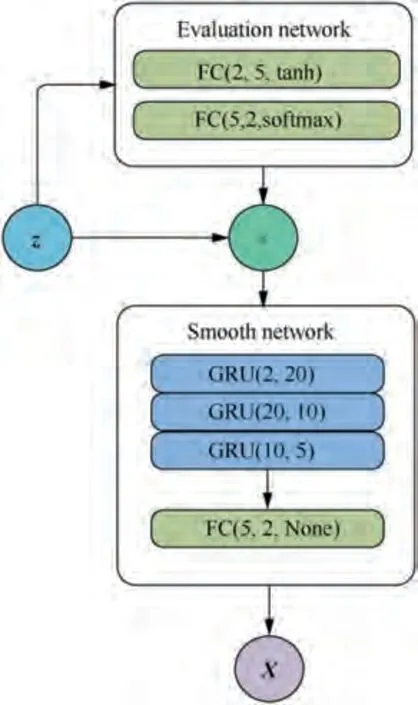
Fig. 13 Specific settings for the two unified filtering neural networks.

As shown in Fig. 13, the two unified filtering neural networks use the same parameter settings.In the part of the evaluation network, the number of neural neurons in the hidden layer is 5, and the activation function is the softmax function.In the part of the smooth network, the number of neural neurons in a three-layer gated recurrent unit is 20, 10, and 5,respectively. Moreover, the number of neural neurons in the fully connected layer is 2, and the activation function is None function.The two unified filtering neural networks are trained in order according to Fig. 12 based on the same training data set,which includes three modes,that is,CV,CA,and CT,each containing 5000 samples, and the total number is 15000. The data structure of the samples in the training data is similar to（x，y）,in which x is the actual input of the filtering network and composed of 20 sequential position measurements about the same target from the same radar,and y is the expected output of the tracking filter network and consists of the real target position sequence corresponding to the radar measurement sequence x. In the process of specifical training, the training data set is divided into a training set and a verification set according to a ratio of 19:1. Additionally, the root means square loss function and the Adam optimizing approach method are adopted. The number of batch training samples is 10, and the number of whole training is 20.

When implementing α-β and Kalman,please refer to Ref.[1]for the initialization methods of target state and covariance,as well as the calculation method of radar measurement covariance. The other related parameters are set as follows.The coefficient of α-β is set to α=0.5， β=0.5, the covariances of the process noises for three different Kalman filters,indicated as CV-Kalman, CA-Kalman, and CT-Kalman, are set to Q=diag（［25，25］）, Q=diag（［100，100］）, and Q=diag（［100，100，0.0001］）, respectively. The LSTM in the LSTM-Kalman filter is set and trained according to Ref. [16].

4.2. Simulation results

The training error curves of the two unified filtering neural networks are shown in Fig.14.It can be seen that both the velocity and position networks have been trained well. The solidline curve for the training loss and the dashed-line curve for the verification loss converge stably and coincide well, which indicates that the training variance of the network is small,and the performance is stable.

In accordance with the generation method of the training set, test data is produced to compare the performance of the unified tracking filter with those of the compared filters. The actual tracking effects of different tracking filters on typical samples from the test set are shown in Fig. 15. Correspondingly, the estimation errors of the target position are shown in Fig. 16, and the estimation errors of the target velocity are shown in Fig. 17.

From the above figures, it can be seen that the unified tracking filter can estimate the target state including position and velocity effectively using the noise radar measurement,which is the same as those of typical filters such as α-β,Kalman, and LSTM-Kalman. The comprehensive analysis and comparisons in Figs. 15-17 show that when the target motion is in CV mode,the performance of the unified tracking filter is better than that of α-β and inferior to those of CV-Kalman and LSTM-Kalman in terms of target position estimation.When the targets motion is in CA mode, the performance of the proposed filter is comparable to that of LSTM-Kalman and superior to those of α-β and CA-Kalman.When the targets motion is in CT mode, the performance of the proposed filter is slightly better than that of LSTM-Kalman and much better than those of α-β and CT-Kalman. In addition, no matter which mode the targets motion is in,the estimation performance of the proposed filter is significantly better than those of the compared filters in terms of target velocity estimation. Therefore, according to the tracking effect on a single sample, in terms of the position estimation performance, the proposed filter is equivalent to the compared filters, but in terms of the velocity estimation performance,the proposed filter is better than the compared filters.

Next, the mean square errors of the position and velocity estimations for different filters are statistically calculated respectively based on the CV, CA, and CT parts of the test set and the entire test set.Further,with respect to α-β,which is adopted as the baseline method, the improvement percentages on performances of different filters are calculated according to （1-MSE/MSE）×100. After calculation and statistics, results are shown in Table1, Table2, Fig. 18, and Fig. 19.

Table 1 and Fig. 18 show the performance comparison on target position estimation. When the target motion is in CV mode, the performance of the UTF increases by 12.93% and is better than those of α-β and CA-Kalman, but compared with 17.04% improvement of CV-Kalman, 17.32% improvement of CT-Kalman, and 17.32% improvement of LSTMKalman, there is a slight gap between the proposed filter and the compared filters. However, when the target motion is in CA mode, the performance of the UTF increases 13.25%,which is optimal by comparison with 9.43% of CV-Kalman,-6.03% of CA-Kalman, 12.87% of CT-Kalman, and 13.01% of LSTM-Kalman. Although CA-Kalman is a matched filter for CA mode, it has the worst performance due to the short measurement time (only 20 s) and slow convergence speed. When the target motion is in CT mode, the performance of the UTF increases 16.84%, which is superior to -67.22% of CV-Kalman, -11.16% of CA-Kalman,-40.88% of CT-Kalman, and 14.25% of LSTM-Kalman.Similarly, the improved performance of CT-Kalman is not good due to the slow convergence speed. In general, for slow-moving targets,the unified tracking filter is slightly lower than the optimal estimation among the compared filters, but above the average level. However, for fast-moving targets, its performance is better than those of the compared filters,which shows that the proposed filter has a well-filtering capability for a maneuvering target. On the entire test set, without knowing the target motion mode in advance, the performance of the UTF increases 14.39%, which is significantly better than-1.34% of CV-Kalman, -7.93% of CA-Kalman, -7.96%of CT-Kalman, and 4.73% of LSTM-Kalman. In addition, it shows that the proposed filter has strong adaptability to different target moving modes. As it can be seen from Table 2, in terms of target velocity estimation, whether in a CV, CA, or CT single-mode test or a three-mode mixed test, the performance of the UTF increases 60%, which is superior to those of the compared filters.

Aiming at the corresponding problem, the compared filters can improve their performances by debugging the parameters

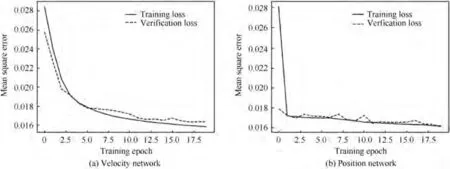
Fig. 14 Training curves of the two unified filtering neural networks.

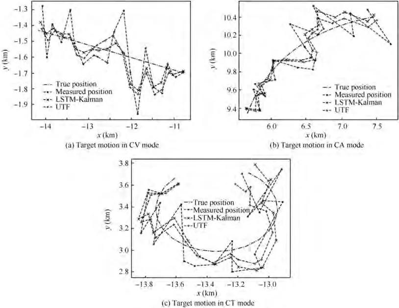
Fig. 15 Actual target tracking effects of different tracking filters.

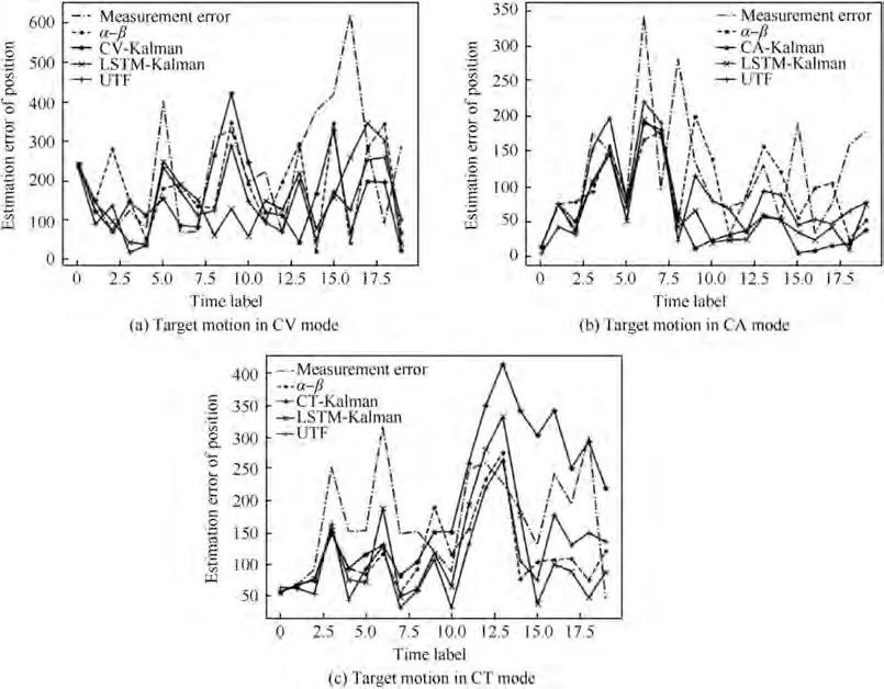
Fig. 16 Comparison on estimation errors of target position between different filters.

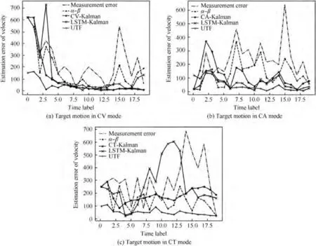
Fig. 17. Estimation errors comparison of target velocity between different filters.

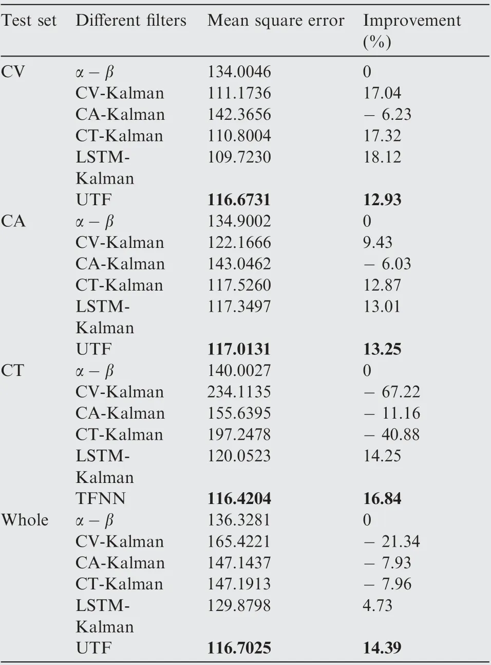
Table 1 Performance comparison on target position filtering.

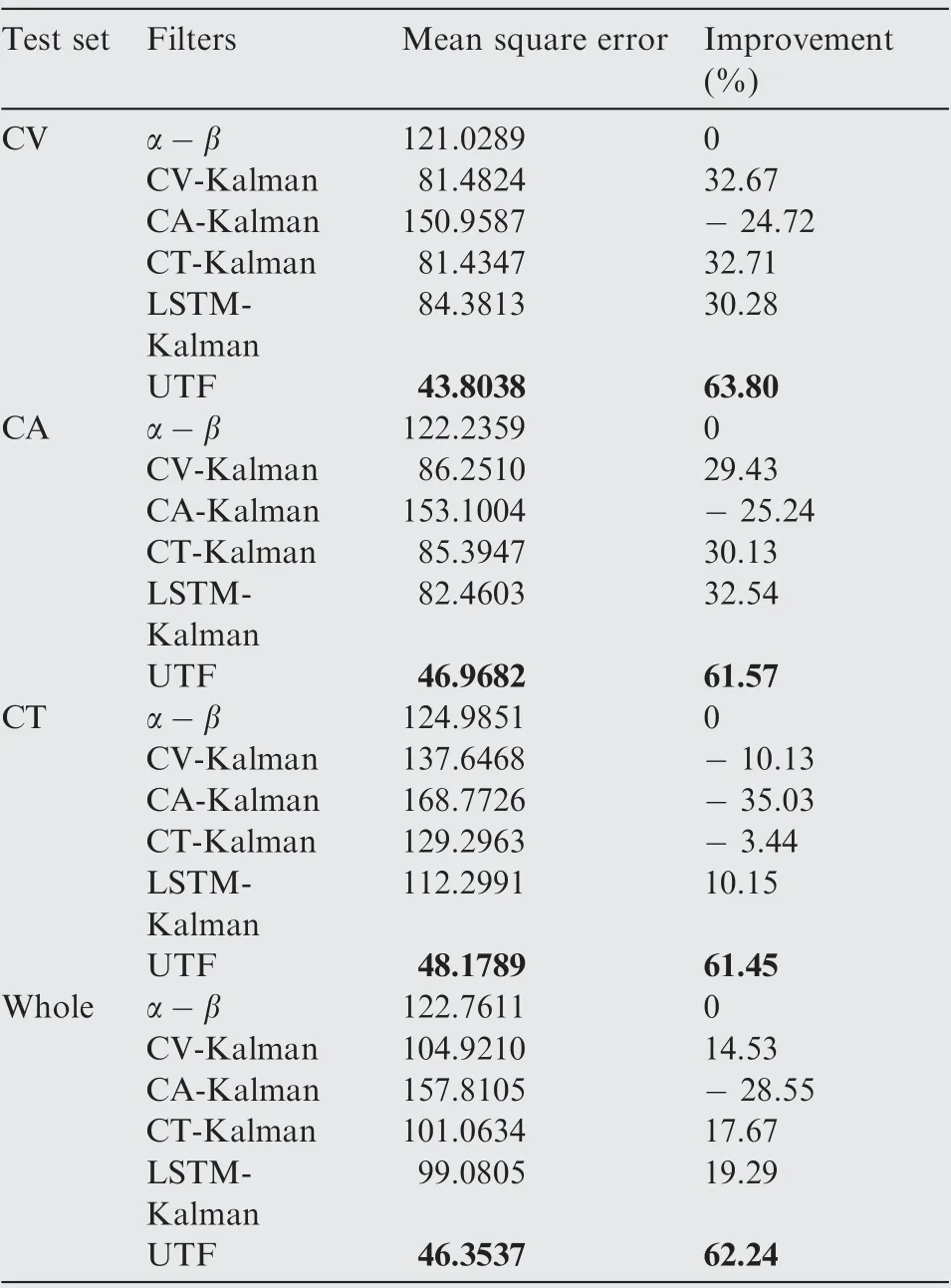
Table 2 Performance comparison on target velocity filtering.

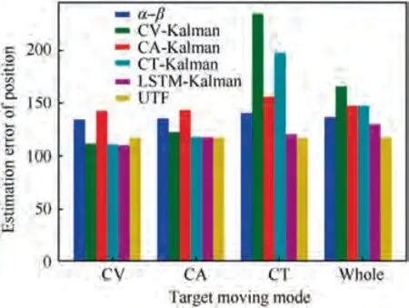
Fig. 18 Performance comparison on target position filtering.

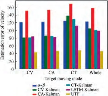
Fig. 19 Performance comparison on target velocity filtering.

(2) Through comprehensive comparison and analysis,it can be concluded that the nonlinear operation in the filter can be expressed as a feedforward neural network structure, the delayed feedback as a constrained recurrent neural network structure,and the filter gain as an attention mechanism. Therefore, a unified tracking filter can be constructed based on basic neural network modules,such as feedforward neural network, recurrent neural network, and attention mechanism.

(3) Experimental validation shows that compared with typical filters,the unified tracking filter is in the middle level and acceptable for slow-moving targets, but has superiority for fast-moving targets in terms of target position estimation. Moreover, the unified tracking filter has an advantage in terms of target velocity estimation. Therefore, the unified tracking filter has good performance and advantages overall.

(4) The proposed filter achieves unity in three aspects,i.e.,a unified target motion model,an adaptive filter,and a filtering framework.

The authors declare that they have no known competing financial interests or personal relationships that could have appeared to influence the work reported in this paper.

This study was supported by the National Natural Science Foundation of China (Nos. 61790554 and 62001499).repeatedly. However, without using the L1, L2, or dropout regularization method, trying other neural network weight optimization methods,and adjusting the number of the neural network layer and the number of neural units, the unified filtering neural network also does not achieve the optimal after just 20 times training. Therefore, the experimental result can show that the performance of the unified filtering neural network can reach or even exceed those of the compared filters without too much debugging and adjusting. In addition, from the perspective of engineering applications, the proposed filter is easier for engineers to use and more convenient for rapid deployment than the compared filters.

Through the above experiments, the feasibility, effectiveness, and advancement of the unified tracking filter have been verified.Hence,the unified tracking filter has potential to get a better filtering effect than those of the compared filters.

5. Conclusions

(1) By constructing and analyzing the structures of typical filters like and Kalman, and making analogies to other filters, it can be found that the delayed feedback structure is the key to realize filtering.Hence,by constructing a more general delayed feedback structure, a filter in a more unified form and with a stronger performance can finally be realized.