Continuous-Time Prediction of Industrial Paste Thickener System With Differential ODE-Net

Zhaolin Yuan, Xiaorui Li, Di Wu, Xiaojuan Ban, Nai-Qi Wu,,Hong-Ning Dai,, and Hao Wang,

Abstract—It is crucial to predict the outputs of a thickening system, including the underflow concentration (UC) and mud pressure, for optimal control of the process. The proliferation of industrial sensors and the availability of thickening-system data make this possible. However, the unique properties of thickening systems, such as the non-linearities, long-time delays, partially observed data, and continuous time evolution pose challenges on building data-driven predictive models. To address the above challenges, we establish an integrated, deep-learning, continuous time network structure that consists of a sequential encoder, a state decoder, and a derivative module to learn the deterministic state space model from thickening systems. Using a case study, we examine our methods with a tailing thickener manufactured by the FLSmidth installed with massive sensors and obtain extensive experimental results. The results demonstrate that the proposed continuous-time model with the sequential encoder achieves better prediction performances than the existing discrete-time models and reduces the negative effects from long time delays by extracting features from historical system trajectories. The proposed method also demonstrates outstanding performances for both short and long term prediction tasks with the two proposed derivative types.

I. INTRODUCTION

AS a core procedure in modern mineral separation, a thickening process produces a paste with high concentration for subsequent tailing storage or backfilling[1]–[3]. During this thickening process, an industrial paste thickener achieves solid–liquid separation based on gravity sedimentation. The purpose of the industrial paste thickener is to efficiently control the final underflow concentration (UC).Most closed-loop control systems manipulate the underflow slurry pump speed and flocculant pump speed as the inputs to stabilize the underflow concentration within its specified range during operation. Previous studies [4], [5] showed that model prediction control (MPC) can facilitate the control process of thickening systems owing to the advantages of its high robustness and applicability. Hence, the accurate prediction of thickening systems has received extensive attention for the analysis and control of thickeners [5]–[7].

A complex industrial system such as the thickening system typically has the following key features:

1) Non-Linear System Dynamics:Most industrial systems have extremely complex high-order dynamical equations that are not affine or linear systems.

2) PartiaLly Observed Data:The information extracted from sensors or other available methods is incomplete. In particular, a number of unknown hidden variables exist in such systems.

3) Influence of Long Delays:The system states are influenced by external inputs or internal states that occur over a long previous time.

4) Continuous-Time (CT) Evolution:Because real industrial systems follow various physical laws, their time evolution can be expressed via CT differential equations.

The above features of a thickening system create challenges for predictive control. There are a number of studies addressing these challenges. Data-driven methods are emerging as one of the most successful techniques for modeling complex processes [8]. Traditional data-based CT system prediction methods focus on fitting high-order differential equations based on sampled noisy data from real systems. However, they lack the ability to cope with partially observed and extremely complex system dynamics. Recent advances of deep neural networks (DNNs) have shown their strengths in addressing these issues owing to their strong feature representation abilities and scalable parameter structures, leading to the wide usage of DNNs in computer vision [9]–[11], natural language processing [12], [13], time series prediction [5], [14]–[17], and fault diagnosis [18].However, most DNN-based system-modeling methods are based on discrete time, disregarding the CT properties of a system. The lost prior information from physical insights undoubtedly leads to the deterioration of the model accuracy.

Studies of prediction control can be categorized into two types. The first type provides short-term predictions for model-based control algorithms [5], such as model predictive control (MPC). The learned system provides deterministic prior knowledge of the dynamical systems, thereby approximating the infinite-horizon optimal control as a shortterm optimization problem. The second type is mainly based on simulations, which imitate the outputs of an unknown system under a long-term feed of inputs [19]. Compared with short-term predictions, simulations require higher robustness and stability to provide long-term predictions. However, there are few studies on designing predictive models for short and long term predictions to support subsequent applications, such as MPC and simulations.

To address the above challenges, we propose a deep CT network composed of a sequential encoder, a state decoder,and a derivative module to learn the auto-regressive processes and influences from the system inputs based on real thickening data in an end-to-end manner. Specifically, the long-time system delay motivated us to utilize a sequential encoder to extract features from historical system trajectories.We designed the derivative module for the CT state space model based on a DNN. This module fits the non-linear CT evolution of the system and infers the non-observable information by introducing hidden states. Moreover, the problems of short and long term predictions are solved by feeding historical system trajectories and system inputs with arbitrary lengths to the model after incorporating the designed non-stationary and stationary systems into the trained model.The future system outputs are then predicted. The contributions of this paper are threefold:

1) We propose a novel deep-learning-based CT predictive model for a paste thickener. The deep learning network consists of three components: a sequential encoder, a state decoder, and a derivative module.

2) We design two kinds of derivative modules, named stationary and non-stationary systems, to handle the shortterm and long-term prediction tasks, respectively.

3) We conduct extensive experiments on real industrial data collected from a real industrial copper mining process. The results demonstrate the outstanding performance of the proposed model in providing predictions for the thickener system with non-linear and time-delay properties. In addition,we conduct ablation studies to evaluate the effectiveness of each module in the proposed model.

The rest of the paper is organized as follows. We briefly introduce the related work in Section II. We then present the problem formulation in Section III. We next present the CT deep sequential model in Section IV. Experimental results are shown in Section V. We then summarize the paper and discuss future research directions in Section VI.

II. PRELIMINARIES AND RELATED WORK

As a core device in a thickening system, a paste thickener is generally composed of a high sedimentation tank and a raking system. Fig. 1 depicts the general structure of a thickener and its key components. After being fed with flocculant and tailing slurry with a low concentration, underflow with a high concentration is discharged from the bottom of the thickener and is then used to produce paste in the subsequent procedures. The prediction of a thickening system refers to the estimation of the future system outputs, such as the underflow concentration and mud pressure based on the historical system trajectories and system inputs. The prediction of a thickening system is essentially similar to system identification [8]. For system identification, interpretable model structures are designed based on prior knowledge, and the parameters are determined by fitting real data. As one of the subsequent applications of identified models, the prediction forecasts the system outputs according to the inputs.

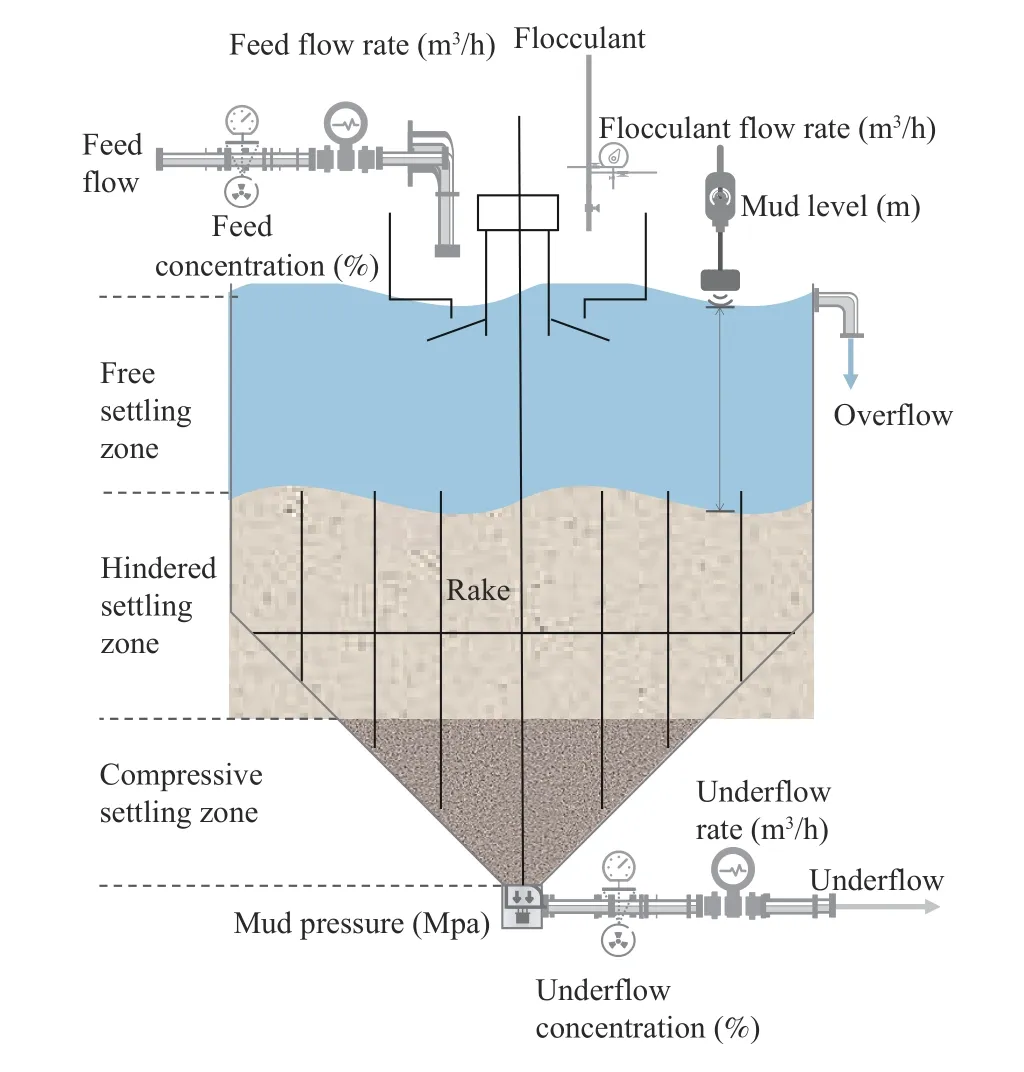
Fig. 1. Crude slurry flow with a low concentration is fed into the mix tank accompanied by flocculant. Under the effect of the flocculant, particles agglomerate to larger clumps and concentrate at the bottom. The paste thickener continuously produces underflow with a high concentration and clear water in an overflow pipe located at the top of the thickener.

A. Prediction of Thickening Systems

The prediction methods for thickening systems can be categorized into two types: 1) gray-box thickening system simulations and 2) black-box thickener system predictions. In the gray-box simulations, the sedimentation process is mainly considered from a physical perspective [4], [20], [21]. Theorybased gray-box methods can be exactly explained and implemented effectively for specific systems. However, most of them are mainly built on many ideal hypotheses and suffer from the complexity of slurry particle dynamics and external unknown environment disturbances.

In contrast, the black-box methods do not require prior assumptions or constraints to be given. A complete parameterized model with a high degree of freedom is defined to predict the system outputs and learn the optimal parameters from real data. Since the offline system trajectories from an industrial system are always available and adequate, blackbox-based methods, including latent factor model [22]–[24],imitation learning [25], and deep neural network [26] have been widely used in the current industrial systems [27]–[32].

Moreover, Oulhiqet al. [33] used a black-box linear dynamic model with a deterministic time delay to identify an industrial thickener system using historical data. Such parameterized linear model lacks adequate expressivity to represent the non-linear properties in a thickening system.Most recently, random forest model is presented for modeling a paste thickening system based on a purely data-driven approach for modeling and evolutionary strategies [34].Because random forest model only fits the thickening system dynamic in single step, it ignores the time delay and the correlations between adjacent positions in sequential inputs and outputs. A bidirectional gated recurrent unit (BiGRU)with an encoder–decoder deep recurrent neural network is introduced to model thickening systems [5]. Yuanet al. [6]proposed a dual-attention recurrent neural network to model the spatial and temporal features of a thickening system,thereby improving the prediction accuracy of the underflow concentration. However, the above studies [5], [6] only focus on discrete-time system predictions rather than a CT thickening system.

B. Prediction of Continuous-Time Systems

The prediction of physical systems based on CT models directly from sampled data has the following advantages [8]:1) transparent physical insights into the system properties, 2)inherent data filtering, and 3) the capability of dealing with non-uniformly sampled data. For any numerical schemes for solving CT differential equations, sophisticated discretization methods have high accuracy but suffer from enormous time and memory costs. A recently developed advanced ordinary differential equation (ODE) solver [35] introduces the reversemode automatic differentiation of ODE solutions, thereby only requiring O(1) memory cost. Meanwhile, this method also allows the end-to-end training of ODEs within a large DNN. Moreover, Demeester [19] proposed a stationary CT state space model for predicting an input–output system when the observations from a system are unevenly sampled.Although it has successfully improved the accuracy and stability of long-term predictions by introducing a stationary system, it did not take advantage of a non-stationary system in the short-term prediction task.

Compared with the existing CT models, our model considers both short-term and long-term predictions, thereby achieving outstanding performance.

III. FORMULATION AND NOTATION OF PASTE THICKENING SYSTEM PREDICTION

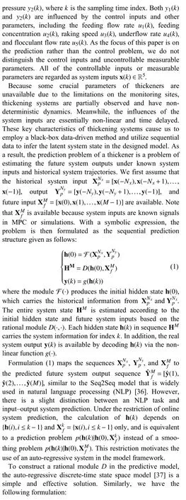
Fig. 2. Proposed model is composed of several components. The recurrent neural network (RNN) encoder outputs the initial hidden state h(t0) according to historical sequences from the system. The derivative module is embedded into the ordinary differential equation (ODE) solver to calculate the hidden state at an arbitrary time. A parallel interpolation mechanism is embedded into the derivative module, which interpolates discrete input sequences to a CT series. Finally,the state decoder module transforms the hidden state to the predicted system output.

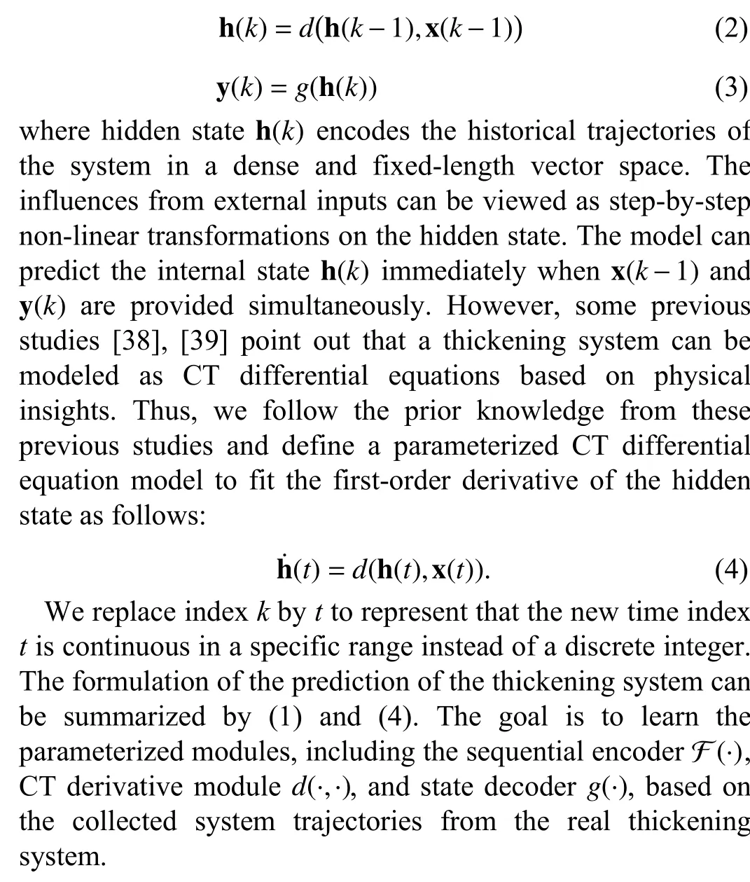
IV. CONTINUOUS-TIME DEEP SEQUENTIAL MODEL FOR THICKENING SYSTEM PREDICTIONS

A. RNN for Encoding Historical Sequences

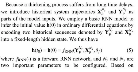
industrial experience, we use the system delay as prior knowledge denoted byTd. If we assume a uniform sampling of the sensors for a sampling intervalTs,NyandNxcan be estimated according to the equationNy=Nx=N=Td/Ts.The influence of parameterNon the model accuracy is examined in Section V. In the thickening system, the correlations between the current system state and historical trajectories are mostly compressed in the short term. This property encourages us to use a simple and unidirectional RNN to encode the historical trajectories of a thickening system. The solved hidden state h(t0) from encoder involves all necessary information of historical trajectories and is represented as an initial state of solved ODE.

B. ODE Solver for Modeling State Space

We employ the parameterized CT state space model to represent the relations between the system inputs, hidden states, and outputs:

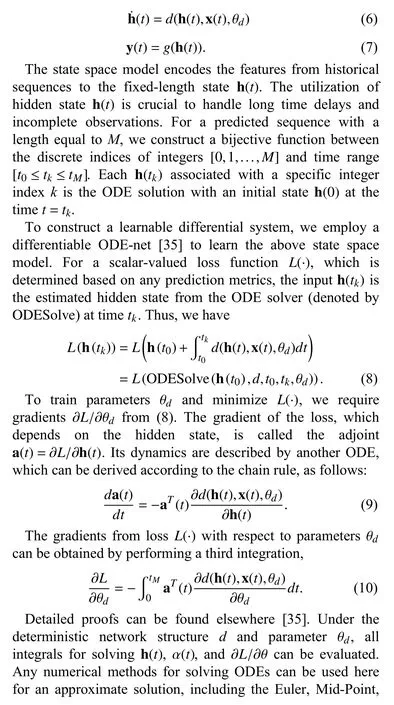
Generally, an ODE solver with a lower error tolerance increases the frequency for calling differential functiond. It leads to more time consumption but results in a higher accuracy. This guideline is also tenable when we construct a neural ODE network to fit sequential datasets. The detailed comparisons of the time cost and accuracy are shown in Section V.

It is worth investigating the definition of a suitable structure ofd. The most intuitive solution is to employ a basic neural network to estimate the derivative that is named nonstationary model.

Non-Stationary:

where MLP(·) denotes a multi-layer perceptron. The combination of a non-stationary system with an ODE solver has a strong similarity to residual connections, which have been widely used in other advanced deep networks [35].

In the field of stochastic process analysis, non-stationary systems are a stochastic process with a mean and covariance that vary with respect to time [40]. Differencing [41] is an effective way to make non-stationary time series stationary by eliminating trend and seasonality. Generally, a thickening system has strong trends in the underflow concentration, mud pressure, and other core variables. The thickening system is an approximation of non-stationary systems, indicating that the differencing operation can improve the fitting accuracy. In(11), the derivative module intrinsically learns the first-order difference of the hidden states in the latent space. In contrast to the operation of differencing the system outputs directly, a model that differences the hidden states has an equivalent or stronger ability to represent a non-stationary system that is of first or even higher order. However, the non-stationary system(11) also suffers from a severe problem when handling longterm prediction tasks. To solve an ODE over long intervals,repetitive accumulation in a CT range can lead to a significant magnitude increase of the hidden states. Consequently, the estimation error will grow accordingly, resulting in the difficulties in achieving accurate system output from the decoder.

Therefore, we devise another derivative module, namely,the stationary system, to handle the long-term prediction problem. In particular, we have

Stationary:

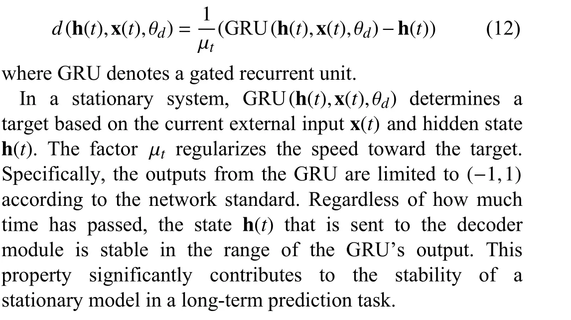
In a stationary system, we use a GRU to construct the derivative module because it has a strong ability to carry longtime information. In a non-stationary system, consecutive accumulations diffuse the hidden state in an unconstrained range. Thus, we employ the MLP to learn the first-order difference h˙(t) directly under h(t) and x(t).

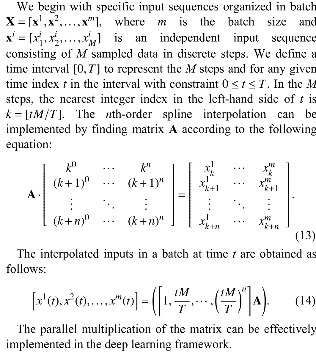
C. Parallel Spline Interpolation

Note that the calculation of h˙(t) in (11) and (12) depends on the external input x(t), which may not exist in our dataset.External input sequences XMfin the training data are discrete,while the computation of the ODE needs x(t) in a CT range.Before each forward pass of the network, it is necessary to interpolate the external inputs to the continuous form. Deep networks are typically trained in mini-batches to take advantage of efficient data-parallel graphics processing unit(GPU) operations. Therefore, we implement a parallel spline interpolation mechanism on top of PyTorch, which is a wellknown deep learning framework.

In our dataset, the external input data are evenly sampled,thereby simplifying the implementation of parallel interpolation. To simplify the explanation, we assume that the dimension of the external input is equal to 1.

D. State Decoder

The state decoder mechanism is essentially a fully connected network. We therefore have the following equation to represent the output,

Compared with other state space models that only employ a single matrix for decoding, the nonlinear decoder is chosen because the accumulative form in (11) causes the range of the input h(t) to be non-deterministic. The activation function tanh(·) constrains the output of the decoder to a rational range.

E. Model Training

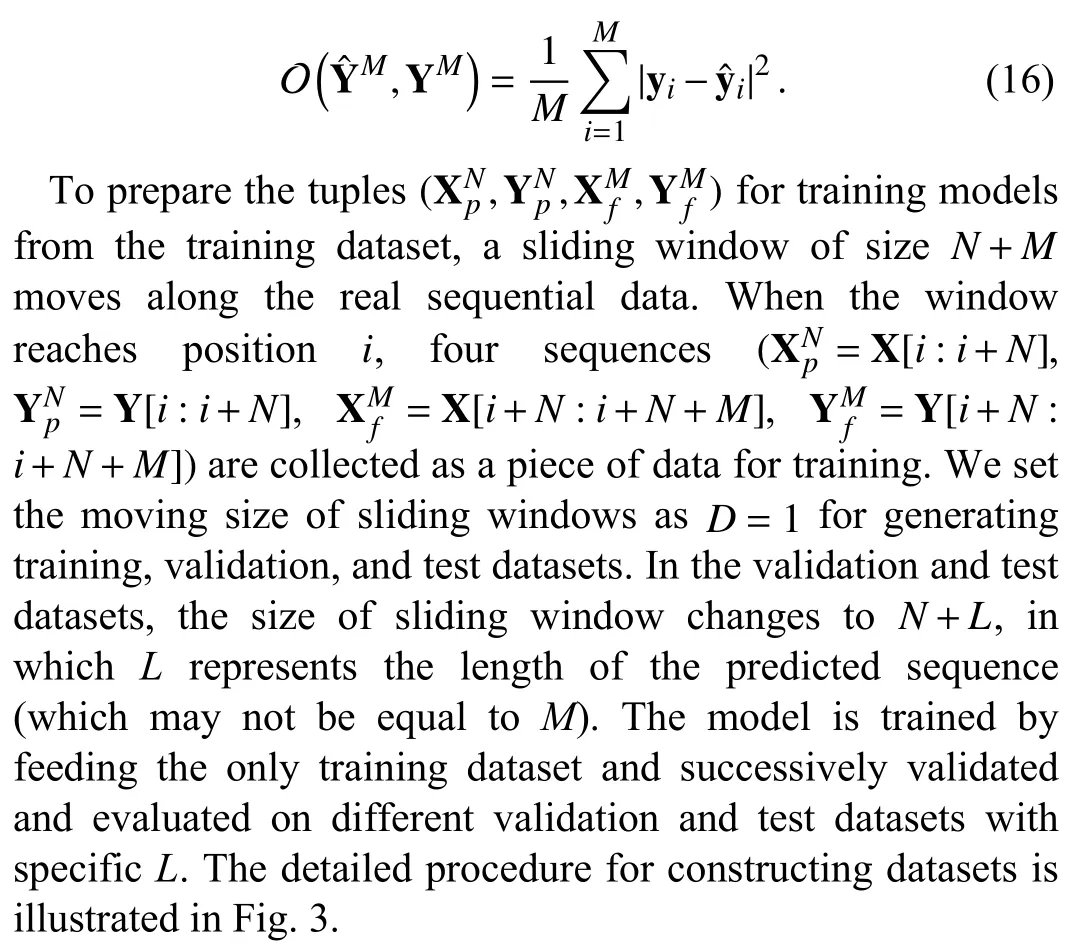
Since all of the operations of the ODE solver in our model are smooth and differentiable, we can train the complete model by the standard back-propagation algorithm with the loss function defined as follows:

V. EXPERIMENTAL RESULTS

This section presents experimental results for the proposed method on the dataset of real thickening systems. We mainly investigate three issues: RQ1: What are the advantages of employing a CT deep sequential network with a high-accuracy ODE solver for modeling a thickening system? RQ2: What are the pros and cons of using stationary and non-stationary systems in prediction tasks? RQ3: How do the different interpolation methods and sequential encoder affect the accuracy of the proposed CT model? We first describe the dataset, the hyper-parameters of the model, and the training and test configurations. We then present the detailed experimental results.

A. Thickening System Dataset

For our experiments, the dataset was collected from the paste thickener manufactured by the FLSmidth from the NFC Africa Mining PLC, Zambian Copperbelt Province. Fig. 4 illustrates two identical thickeners in our experiments. They are used to concentrate copper tailings to produce paste in the backfilling station. Both devices operate in the closed-loop mode with PID controllers.

Some key technical parameters of the studied thickener are listed in Table I.

The measured data are sampled evenly with two-minute intervals from May 2018 to February 2019. A short piece of original dataset is shown in Table II. The collected data come from seven monitoring sensors just as the defined y(k) and x(k)in Section III. After deleting the records corresponding to the time when the system was out of service, there are 24 673 pieces of data remaining.

Fig. 3. Illustration of the process of building both the training, validation, and test datasets. An independent data tuple for training or testing is composed of four vector sequences. X[i:i+N] and Y[i:i+N] represent the historical trajectories in conditional range. X[i+N:i+N+M] and X[i+N:i+N+L] represent the inputs sequences, which have equivalent length with predicted sequences. Y[i+N:i+N+M] and Y[i+N:i+N+L] represent the real system outputs. The former is utilized to generate optimized loss in training and the latter is only used in testing and validation phase for evaluating the accuracy of prediction.

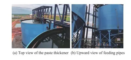
Fig. 4. The figures illustrate two identical paste thickeners in our experimental mining station, including one primary and one alternate thickener. Both devices operate in closed-loop mode with proportionalintegral-derivative (PID) controllers.

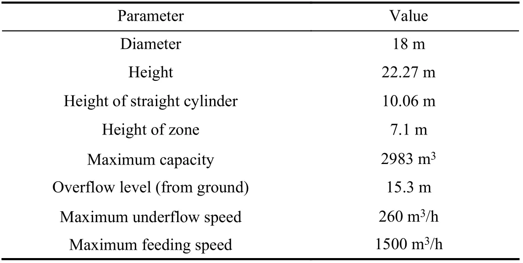
TABLE I SOME KEY TECHNICAL PARAMETERS OF THE THICKENER

We employ the first 70% of the entire dataset to train the model. In the remaining 30% portion, the first 15% is used for validation to determine the best training epochs, and the other 15% is the test dataset for evaluating the model accuracy. By splitting and building the inputs-outputs sequential tuples according to Fig. 3, there are 17 131 tuples left for training and 3561, 3421, 3121 tuples left for testing and validation forL=60, 200, 500, respectively. All the datasets are normalized to standard normal distributions with a unified mean and variance before the training and test phases.

B. Experimental Setup

We use the mini-batch stochastic gradient descent (SGD)with the Adam optimizer [42] to train the models. The batch size is 512, and the learning rate is 0.001 with an exponential decay. The decay rate is 0.95, and the period for decay is 10 epochs. The size of the hidden state h(t) in ODE is 32. The RNN encoder module has a single hidden layer and the size is equal to 32 that is consistent with the size of hidden state h(t).The size of the hidden layer in state decoder is 64. In both the adaptive ODE solvers, the time for solving the ordinary differential equations increases if we reduce the tolerance of approximate error. For balancing the time cost and accuracy,we set the relative tolerance to 1E–4 and absolute tolerance to 1E–5 in all of experiments.

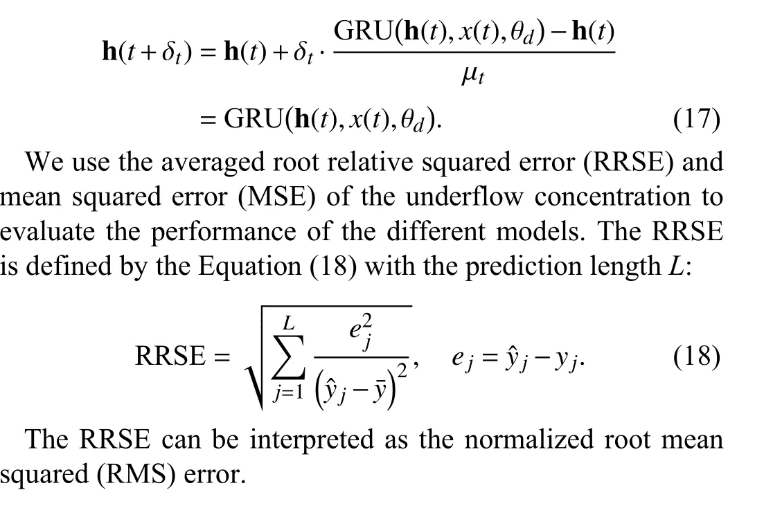
During the training procedure, the length of the historical sequences denoted byNis 80, and the length of predicted outputs denoted byMis 60. The best-performing model in the validation dataset is chosen for further evaluation with the test dataset. The training and test phases were performed on a single Nvidia V100 GPU. The implementation uses the PyTorch framework. We define the CT range as0 ≤t≤Mδtfor given discrete integral indices [0,1,...,M]. The time interval δtof the adjacent data points is set to 0.1.Accordingly, the normalized factor µtin (12) is also set to 0.1.When we use the Euler approximation to solve an ODE equation in a stationary system, the predicted hidden state in the next time step is equal to the output of the GRU cell corresponding to the discrete-time system:

C. Results and Discussion

1) Main Results

We investigate the influence of the types of ODE solversand system types. We select four ODE solvers: Euler, Mid-Point, fourth-order Runge-Kutta (RK4), Dormand-Prince(Dopri5) [35], and 3-order Bogacki-Shampine (Bosh) [43].We investigate the performances of those ODE solvers in both non-stationary and stationary systems. To make a trade-off between the model accuracy and time consumption, we set the relative tolerance to 1E–4 and the absolute tolerance to 1E–5.Moreover, we also consider the discrete-time deep sequential model for the state space (DT-State-Space), the attentionbased Seq2Seq model (Attention-Seq2Seq) [5], and Transformer [44] for comparison. The DT-State-Space [45]model employs a parameterized per-time-series linear state space model based on a recurrent neural network (RNN) to forecast the probabilistic time series. The sizes of state space and RNN hidden layer are set to 16 and 32, respectively. The hyperparameters setting of Transformer and Attention-Seq2Seq are kept with the original literature.

TABLE II A TABULAR EXAMPLE OF PASTE THICKENING SYSTEM DATASET

We conduct three groups of experiments to investigate the RRSEs, MSEs, and time consumption of models with prediction lengths ofL=60, 200, and 500.

a) Comparison of proposed and other baseline models:

We first examine the performance of the Attention-Seq2Seq model, the DT-State-Space model, and Transformer, which are defined in discrete-time settings in Table III. Although they perform competitively, better than the proposed models with the Euler ODE solver, they perform worse than the models with high-order ODE solvers, especially for long-term predictions. The results also indicate that employing a CT model is consistent with the features of the CT evolution in thickening systems, thereby improving the prediction accuracy.

b) Comparison of different ODE solvers:

We analyze the comparisons of different ODE solvers respectively from stationary system and non-stationary system. When the derivative module is defined as a nonstationary system and we only focus on short-term prediction withL=60, we find that the Euler method achieves relatively higher RRSE and MSE values (i.e., poorer prediction performances) than the other four ODE solvers, though it has a much lower time consumption than the other solvers. As the simplest method for solving ODEs, the Euler method evaluates the derivative network only once between two adjacent time points. Meanwhile, the Mid-Point and RK4 methods have higher prediction accuracies than the Euler method, since they evaluate the derivative network two and four times, respectively, between two adjacent time points.Moreover, the Dopri5 and Bosh methods achieve better accuracies, though they have higher time consumptions.Dopri5 performs slightly better than Bosh. As adaptive methods in the Runge-Kutta family, the Dopri5 and Bosh methods ensure that the output is within a given tolerance of the true solution. Their time consumptions for solving an ODE equation increase as the accuracy tolerance is decreased.

Strangely, with the increase in the prediction length, we find that the accuracies of non-stationary models crash gradually and the degradation of Euler is slightly lower than the others.The reason of this inconsistent phenomenon is that nonstationary system brings accumulative errors in long-term predictions. High-order ODE solvers evaluate the derivative module more times recursively, which brings more accumulative errors. Not only do the high-order solvers not improved the accuracies of non-stationary system in long-term predictions, they made the accuracies worse.

When the derivative module is switched to a stationary system. It is worth mentioning that the time consumption for the two adaptive methods, Bosh and Dopri5, to solve an ODE equation significantly increases. We do not list the accuracies of the Dopri5 and Bosh for the stationary systems in Table III because the extremely slow speed makes the method ineffective for practical applications. According to the comparison of the ODE solvers, the high-order ODE solver,such as RK4, results in lower fitting errors than the low-order methods while requiring more time to evaluate the ODE equations intensively.

c) Comparison of stationary models and non-stationary models:

For comparing the distinctions between stationary models and non-stationary models more intuitively, we further visualize the prediction performance of the non-stationary and stationary systems with different ODE solvers. Fig. 5 depicts the predicted sequences of the non-stationary and stationary systems with different ODE solvers for the short-term prediction task withL=60. The results show that the nonstationary models outperform the stationary models in shortterm prediction tasks. The estimated sequences from the nonstationary models are slightly closer to the real system output than those from the stationary models. The learning process of a non-stationary system is essentially equivalent to differencing the hidden state and employing the MLP network to learn the relatively stationary first-order difference.Furthermore, the non-stationary models can predict the system outputs smoothly because the non-stationary structure limitsthe hidden states to only changing in a continuous and slow manner. This constraint is consistent with the properties of a slow thickening system that shrinks the searching space of the model parameters to prevent overfitting.

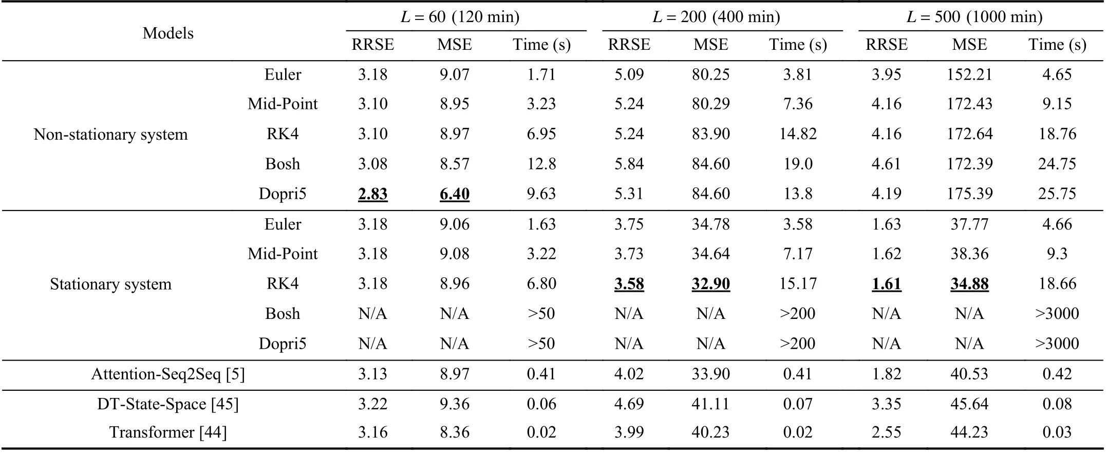
TABLE III ROOT RELATIVE SQUARED ERROR (RRSE), MEAN SQUARED ERROR (MSE), AND TIME CONSUMPTION OF PREDICTED UNDERFLOW CONCENTRATION

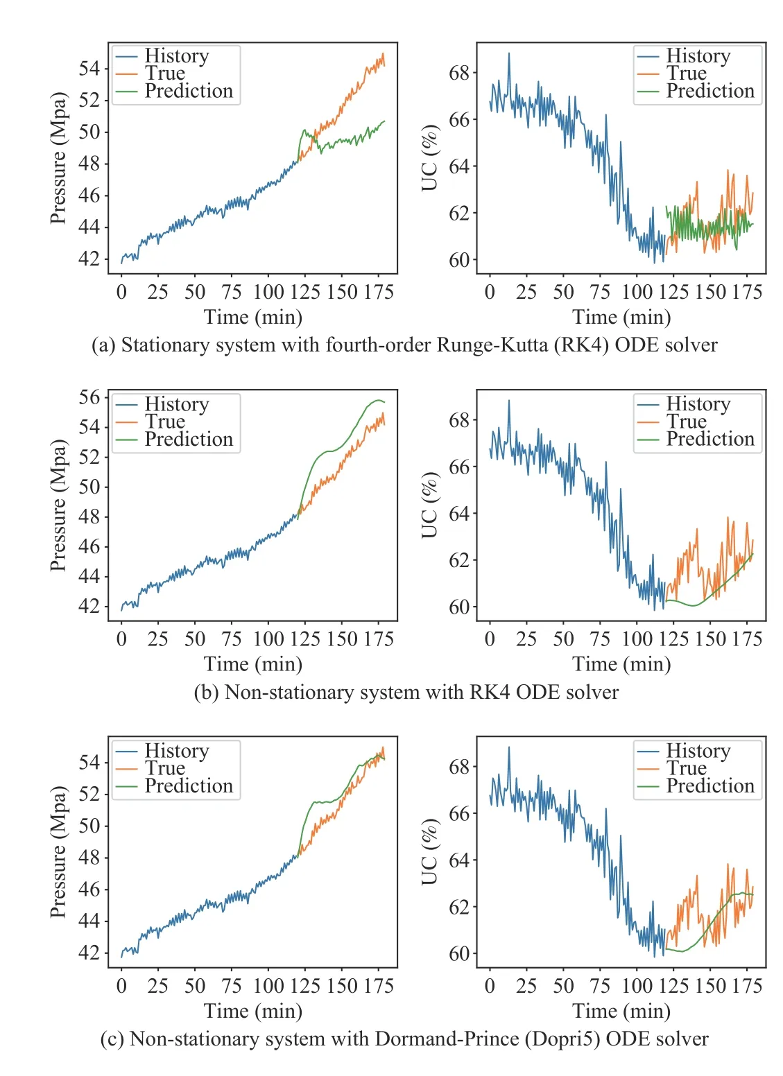
Fig. 5. In the short-term prediction task with L=60, the non-stationary models output more stable and accurate sequences than the stationary models.

Fig. 6 presents the experimental results of a long-term prediction task withL=200 (similar results withL=500 can be found in Table III). The tabular results in Table III demonstrate that the RRSE and MSE of non-stationary models are much higher than those of the stationary ones in long-term prediction task, which is consistent with the graphical results.Compared to the excellent results of non-stationary models in Fig. 5, Fig. 6(a) shows that the prediction accuracy for the non-stationary system decays significantly, and the predicted outputs deviate from the true outputs gradually with the increase in the prediction length. However, the predicted results of stationary models are stabilized and closed to the true system outputs, which confirms the excellent accuracies of stationary models in the long-term prediction problem. The structure of non-stationary ODE leads to the hidden state in progressive evolution that is unconstrained and gradually expanding. Although we embed a tanh function for the decoder network to restrict the final prediction of the underflow concentration and pressure to a rational range, it is impossible for the decoder module to learn an effective mapping function from an extremely large hidden state space to the system output space. Similarly, Fig. 6 also demonstrates that high-order ODE solvers, such as the 4th-order Runge-Kutta, still perform slightly better than the low-order solvers,such as Euler, in long-term prediction.

We conduct five other groups of experiments with different values of the prediction length to evaluate the prediction performance (i.e., the MSE) of the underflow concentration and ground-truth for both stationary and non-stationary systems. The results in Fig. 7 show that the non-stationary system performs better than the stationary system in the shortterm prediction task (e.g.,L<100), although the stationary system outperforms the non-stationary system in long-term prediction tasks. For example, whenLexceeds 120, the errors from the non-stationary system increase with the predicted length, while the stationary system significantly stabilizes the accumulative errors in the long-term prediction.

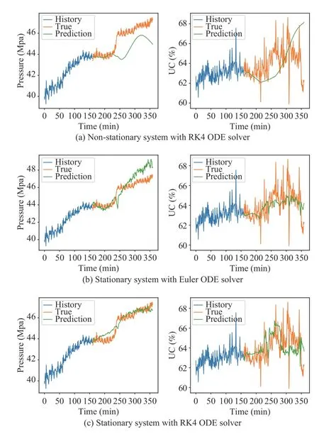
Fig. 6. In the long-term prediction task with L=200, Fig. 6(a) illustrates that non-stationary models only performed well in the early time horizon. In the late horizon, the predicted sequences deviated from the true system outputs significantly compared with those of the stationary models, which are shown in Figs. 6(b) and 6(c). The results also indicate that the models with high-order ODE solvers performed better than the models with low-order ODE solvers in long-term prediction tasks.

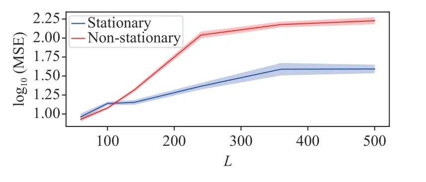
Fig. 7. Predicted length L affected the accuracy (log10 MSE ± 2σ, computed across five runs) of predicted underflow concentration for both stationary and non-stationary systems.

2) Experiments for Evaluating Interpolation Order

We next investigate the effect of the interpolation method on the prediction accuracy. We test four spline interpolation methods with different orders and compare the prediction accuracies on test datasets. The results in Table IV demonstrate that the higher-order interpolations slightly outperform the lower-order ones. This proves that the system input of the thickening system is a non-linear complex process, and that the information from external inputs is essential for predicting the outputs of the system. Higherorder spline interpolations exploit more correlational features from adjacent inputs and interpolate the empty area with a better accuracy than the lower-order interpolations.

3) Ablation Experiments for Studying System Time Delays and Improvements From Sequential Encoder

Finally, we investigate the significance of introducing the sequential encoder to confront the system time delay. We investigate the influence ofNon the model accuracy.Specially, whenNis set to 1, the sequential encoder is replaced by a neural network with one hidden layer that encodes the system output x(k−1) in a single time step to the initial hidden state h(t0). WhenNis set to 0, the initial state h(t0)is a learnable or zero vector [19] that had no relationship with historical system trajectories. We examine the different choices ofNin experiments withL=60, 200, and 500,respectively. In the experiments withL=60, the derivative module is set to be a non-stationary system with an MLP cell.We change it to a stationary system with a GRU cell whenL=200and 500. The ODE solver is the fourth-order Runge-Kutta solver for all of the models.

The results shown in Table V demonstrate that the introduction of the sequential encoder to extract features from the historical sequence leads to better performance than those in the cases withN=1 or 0. The intuitive explanation is that the predicted output sequences have strong statistical correlations with historical system trajectories. The optimal length of the encoded sequence is approximatelyN=80,which is consistent with our prior experience of 2–3-h time delays in thickening systems. When the length of input sequence exceeds the optimal value, the accuracy slightly decreases.

Intuitively, the short-term prediction task benefits more from historical system trajectories than the long-term prediction task. When the length of the predicted sequence increases, the advantage brought by the sequential encoder also decreases. In the task withL=500, the profit of employing sequential encoder decreases obviously.

VI. CONCLUSIONS

This paper focuses on the prediction of the outputs of a thickening system based on deep neural sequence models. We introduce a CT network composed of a sequential encoder, a state decoder, and a derivative module, with internal computation processes including interpolation and a differential ordinary differential equation solver, to describe the complex dynamics of a thickening system. Experiments on datasets from real thickening systems demonstrate that the introduction of the sequential encoder and parallel cubic spline interpolation play a crucial role in our model architecture. We conducted extensive experiments to evaluate the proposed models for both stationary and non-stationary systems with different ODE solvers. The results show that the non-stationary system outperforms the stationary system for short-term prediction tasks. However, the non-stationarymodel suffers from the accumulation of errors from the incremental calculation, thereby leading to inferior results in long-term prediction tasks. This demonstrates that the model with the non-stationary system is more suitable for being embedded in a model-based feedback controller (e.g., MPC controller) while the stationary system avoids this problem and performs better in long-term prediction tasks. Therefore,the model with the stationary system is a better choice when a stable and robust identified system is required to predict longterm sequences (e.g., simulations or controller testing).

TABLE IV ACCURACY COMPARISONS WITH DIFFERENT ORDERS OF INTERPOLATIONS

TABLE V ACCURACY COMPARISONS WITH DIFFERENT METHODS FOR GENERATING THE INITIAL HIDDEN STATE h(t0)

In the industrial data processing field, it is a common requirement to process unevenly spaced data. Although the dataset employed in this paper is sampled evenly, we can extend our method to deal with uneven data naturally by adjusting the time intervals. This extension deserves further experimental verification in future work. Another promising research direction is to extend the method to probabilistic generative models and perturbed time-varying models [46] for determining the unknown sampling noise and uncertainty in thickening systems. Moreover, it is worth investigating our method for other dynamical industrial systems.