A Fusion Kalman Filter and UFIR Estimator Using the Influence Function Method
Wei Xue,, Xiaoli Luan, Shunyi Zhao, Senior, and Fei Liu
Abstract—In this paper, the Kalman filter (KF) and the unbiased finite impulse response (UFIR) filter are fused in the discrete-time state-space to improve robustness against uncertainties. To avoid the problem where fusion filters may give up some advantages of UFIR filters by fusing based on noise statistics, we attempt to find a way to fuse without using noise statistics. The fusion filtering algorithm is derived using the influence function that provides a quantified measure for disturbances on the resulting filtering outputs and is termed as an influence finite impulse response (IFIR) filter. The main advantage of the proposed method is that the noise statistics of process noise and measurement noise are no longer required in the fusion process, showing that a critical feature of the UFIR filter is inherited. One numerical example and a practice-oriented case are given to illustrate the effectiveness of the proposed method. It is shown that the IFIR filter has adaptive performance and can automatically switch from the Kalman estimate to the UFIR estimates according to operating conditions. Moreover, the proposed method can reduce the effects of optimal horizon length on the UFIR estimate and can give the state estimates of best accuracy among all the compared methods.
I. INTRODUCTION
TO estimate the states of industrial systems, including power electronic systems, large-scale systems, cyberphysical systems, static neural networks and motion control systems, state estimators are considered to be a fundamental tool [1]–[5]. Kalman and Bucy proposed the famous Kalman filter (KF) in the 1970s [6], which is a simple and globally optimal state estimator for linear Gaussian processes [7]. Up until now, it has been widely used in numerous areas with great success. Given an accurate linear model, the KF can theoretically reach optimal estimates [8]–[10], while its errors will rise dramatically once the underlying model is slightly mismatched or there is colored noise. Due to the complexity industrial processes, it is difficult and time-consuming to find an accurate filtering model, and more importantly, the random external interference barely obeys the Gaussian and white statistics. Therefore, many efforts have been made during the last two decades to improve KF performance under different environments [11]–[14].
As a type of finite impulse response (FIR) filters, the unbiased finite impulse response (UFIR) filtering algorithm is constructed and analyzed in [15]. This algorithm ignores the statistical characteristics of noise sources and initial distribution and uses an optimal estimation interval to drive estimation accuracy to approach its optima in the minimum mean square error sense [15]–[17]. Unlike the KF, which recursively computes state estimates, the UFIR filter operates with a finite number of most recent data either in a batch form or in an iterative structure. Therefore, the UFIR filter accumulates estimation errors only within a limited horizon[18]–[21]. Under harsh industrial operating conditions, it is expected that the UFIR filter exhibits better robustness against uncertainties and will be insensitive to changes in the noisy environment. A detailed comparison of the UFIR filter and the KF is provided in [22], [23] with practical examples.
As discussed, each filtering algorithm has its features.Specifically, the KF provides the best linear estimates (or almost the best) when the underlying linear model is accurate or nearly accurate, while the UFIR estimator shows impressive robustness against uncertainties. With the boom in the development of both filters comes a variety of fusion strategies. There are self-fusion strategies for the same filter to make better use of the characteristic of the filter [24], [25]. If one wishes to design a filter to achieve the optimality of the KF and the robustness of the UFIR filter simultaneously, a common practice is to find an appropriate strategy to fuse them. For example, an infinite impulse response (IIR)-type filter and an FIR-type filter are merged in [26] using the mixing probability calculated based on the residuals and their covariances. Later, in [27] the KF and UFIR filters are fused by assigning probabilistic weights to achieve smaller errors.With the same motivations, the weighted UFIR filter is derived using the Frobenius norm in [28], [29]. Reference [30]uses measurement differencing and by de-correlating noise vectors to fuse the two filters. A unified fusion framework employed in these approaches is demonstrated in Fig. 1,implying that the IIR and FIR filters give respective estimates,and a fusing procedure then achieves the overall output.
Although this structure is clear and pellucid, fusing the UFIR estimate and the Kalman estimate mathematically may not be as intuitive as Fig. 1. The main difficulty is that the
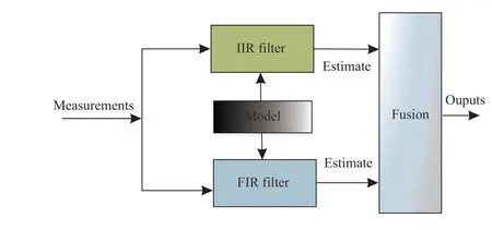
Fig. 1. A diagram of the state vector fusion framework for the IIR-type filter and the FIR-type filter.
II. PRELIMINARIES AND PROBLEM FORMULATION
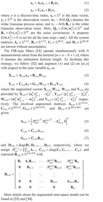
The state-space model provides us with a useful tool to describe an industrial process, where the internal state variables are the smallest possible subset of system variables that can represent the entire state of the system at any given time. Consider a linear discrete-time state-space model specified as error covariance of each filter and their cross-covariance matrix are necessary [26], [27] to conduct fusion, while these prerequisites will destroy the advantages brought by the UFIR filter. To be specific, noise statistics are unavoidable to get error covariances of the UFIR filter, which, on the contrary,ignores the noise statistic completely to get state estimates.Accordingly, one faces a dilemma that for robustness, we hope to avoid using noise statistics, which have to be introduced in the existing approaches [28] for fusion. Besides,it is well known that the KF is recursive while the UFIR filter operates either in batch or in an iterative form, causing further challenges to fuse them without error covariances.
To solve these issues, in this paper we propose a novel fusion procedure, which is designed particularly for the KF and the UFIR filter. The resulting method is constructed based on a concept of an “artificial” filter gain for the UFIR filter as well as the influences function [31]. Compared to the existing fusion methods proposed, the most significant contribution of our paper is that it does not use the statistics of noise. It demonstrates that the critical feature of the UFIR filter is ultimately inherited. Other contributions of this paper are as follows. 1) The proposed algorithm serves as a new fusion approach to fuse the UFIR filter and the KF without calculating error covariances; 2) The proposed method inherits the advantages of the KF and UFIR filter, and can automatically prioritize its performance towards optimality or robustness to accommodate its operating environment; 3)Since noise statistics are no longer required in the fusion step,the proposed method is insensitive to the statistical error of noise and yields significant improvements over existing fusion methods in different scenarios.
The remainders of this paper are organized as follows. In Section II, some preliminaries are given, where we also formulate the problem considered. In Sections III, we propose the fusion algorithm by introducing artificial gain for the UFIR filter and using the influences function approach.Section IV presents the simulation results for several examples, and conclusions are summarized in Section V.
The following notations are used throughout the paper.RNdenotes theN-dimensional Euclidean space,E{·} denotes statistical averaging, diag(D1D2···Dn) represents a diagonal matrix with diagonal elements D1,D2,...,Dn, I is the identity matrix of proper dimensions, A⊙B denotes the Hadamard product of A and B, and A/B is the element-wise division.
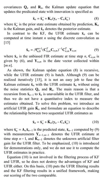
A. Kalman Filter and UFIR Filter

B. Problem Formulation
The problem considered in this paper can now be formulated as follows. Given the Kalman estimate and the UFIR estimate at each step, we would like to design a filter fusing them without involving the estimation error covariances. Besides, we would also like to test the effectiveness of the proposed method by different scenarios and show its trade-off between the existing fusion approaches through applications.
III. FUSION KALMAN/UFIR FILTER
In this section, we propose a novel algorithm to fuse the Kalman and UFIR estimates without using the process noise and measurement noise covariances. The key idea is to run the KF, and the UFIR filter in parallel to produce two different state estimates and then assign weights to these sub-estimates to get the overall outputs. Consequently, determining how to calculate the weights appropriately without noise statistics is essential, and the existing fusion approaches [27], [28]become invalid in this scenario.
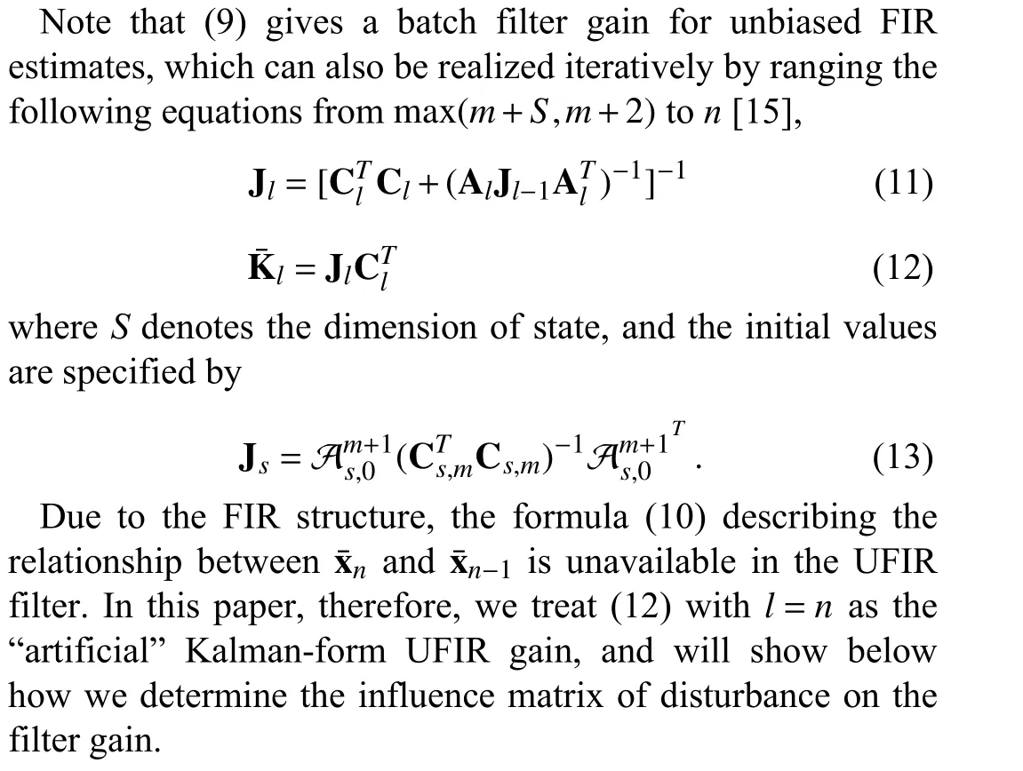
A. Artificial UFIR Gain
B. Influence Matrix
The function of the influence matrix is to quantify how much the filter is affected by disturbances at a given moment.The value of the matrix reflects the robustness of the filter.
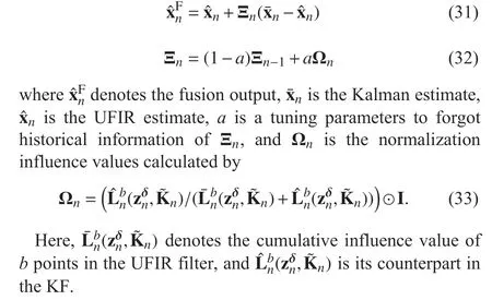
As discussed, the KF needs to know the exact noise statistics to get the state estimates, whereas the UFIR tracks the mean value of the state, implying that noise information is no longer needed. Because of these, we first measure the amount that the same disturbance will affect the estimated value in each filter using the influence matrix.
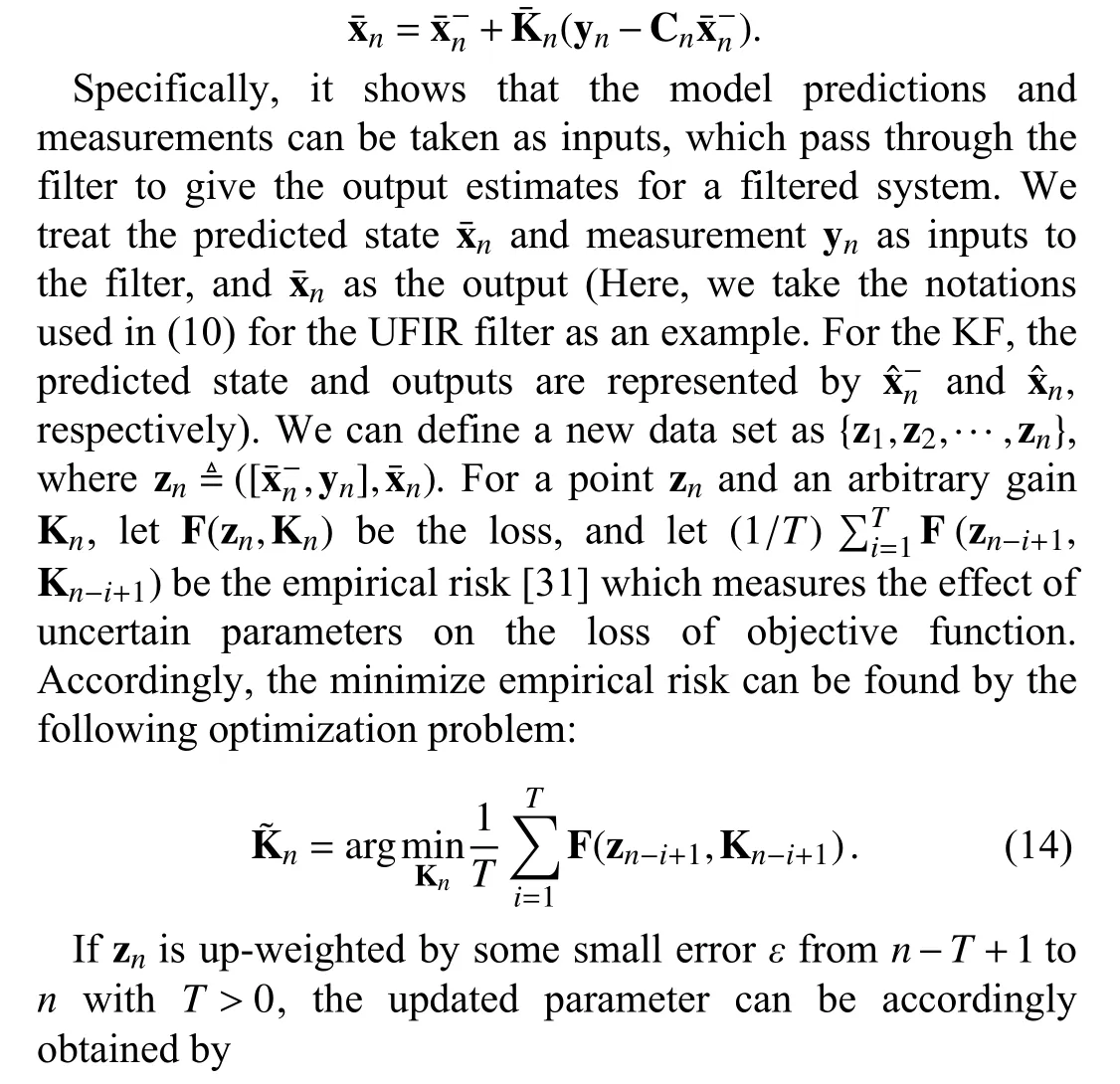
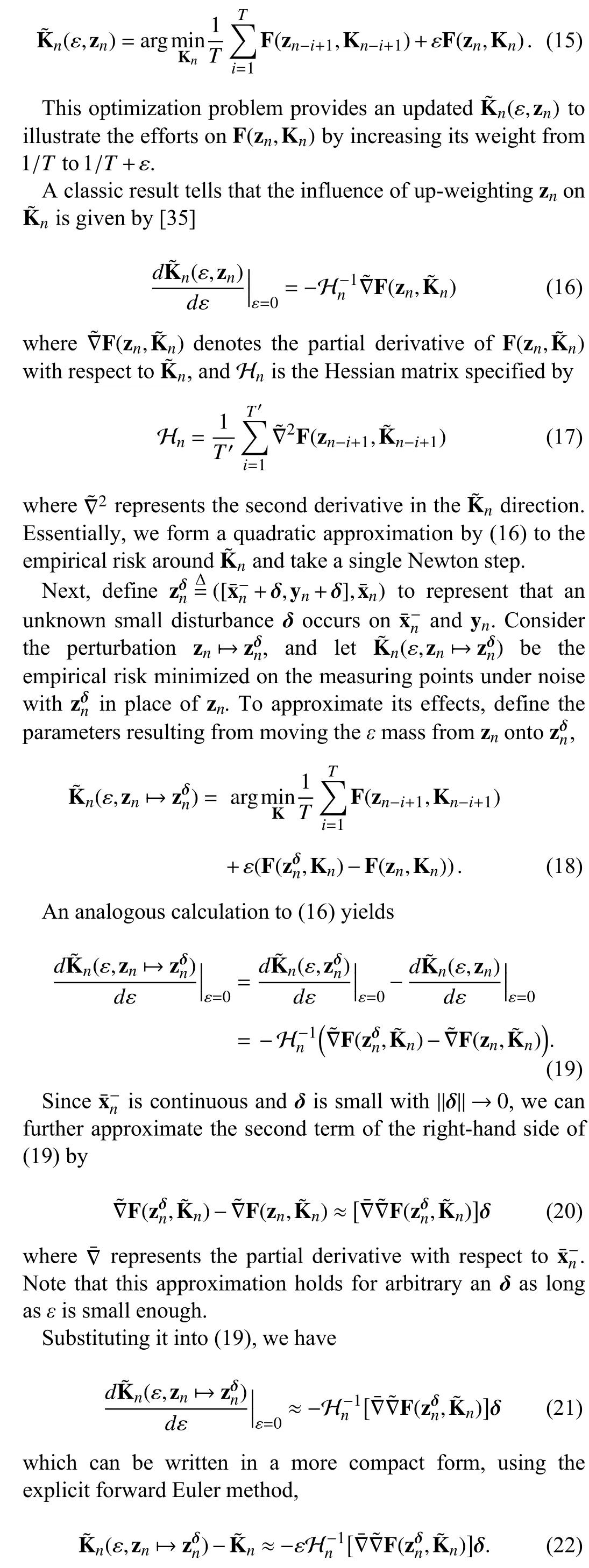
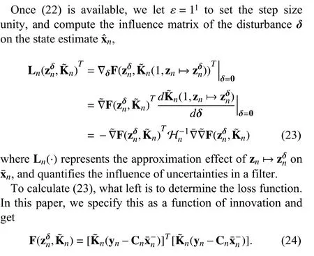
Consider (8) and (10) that map the predicted state and measurement to the filtered state. A filter is, in a way, used to balance the observed and model-predicted values. For a given time, the filter can be seen as the system shown input-output as
C. Cumulative Influence Matrices
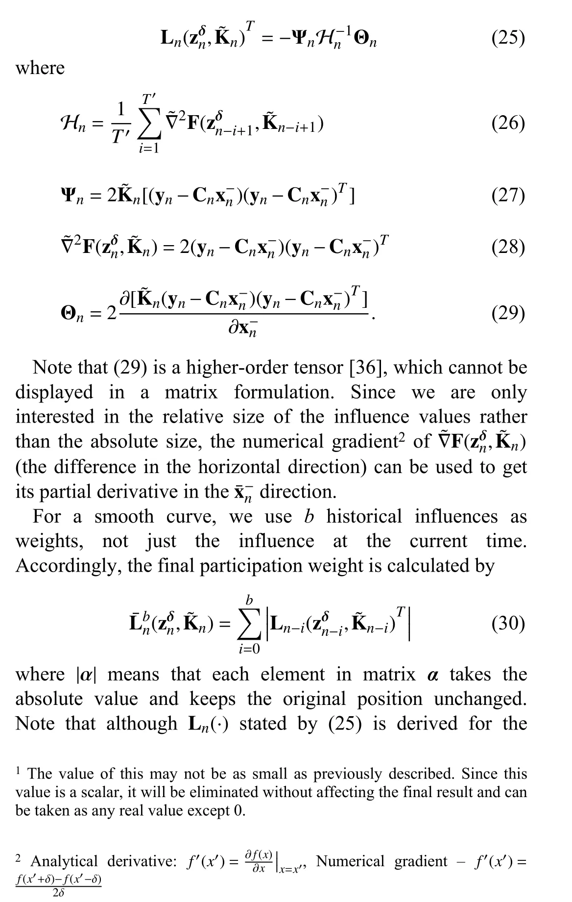
Using (23) and (24), we can get the influence value of disturbance in the UFIR estimates as

D. Fusion Outputs
Now, a rule of thumb for fusion is that the greater the influence is, the greater the degree of noise interference.Consequently, the output should be closed to the estimates with small influence value as much as possible, resulting in
E. Discussions
Algorithm 1 presents the pseudo-code of the proposed method to fit the corresponding block diagram shown in Fig. 2.Fig. 2 represents the structure of the influence finite impulse response (IFIR) algorithm. Firstly, KF and UFIR are run independently to obtain the estimates and gain, respectively.The influence function is then used to obtain the fusion weights. Finally, the two estimates are fused based on the fusion weights. The significant difference when compared to existing fusion algorithms is that the statistical parameters of noise are missing from the input to calculate the fusion weights.
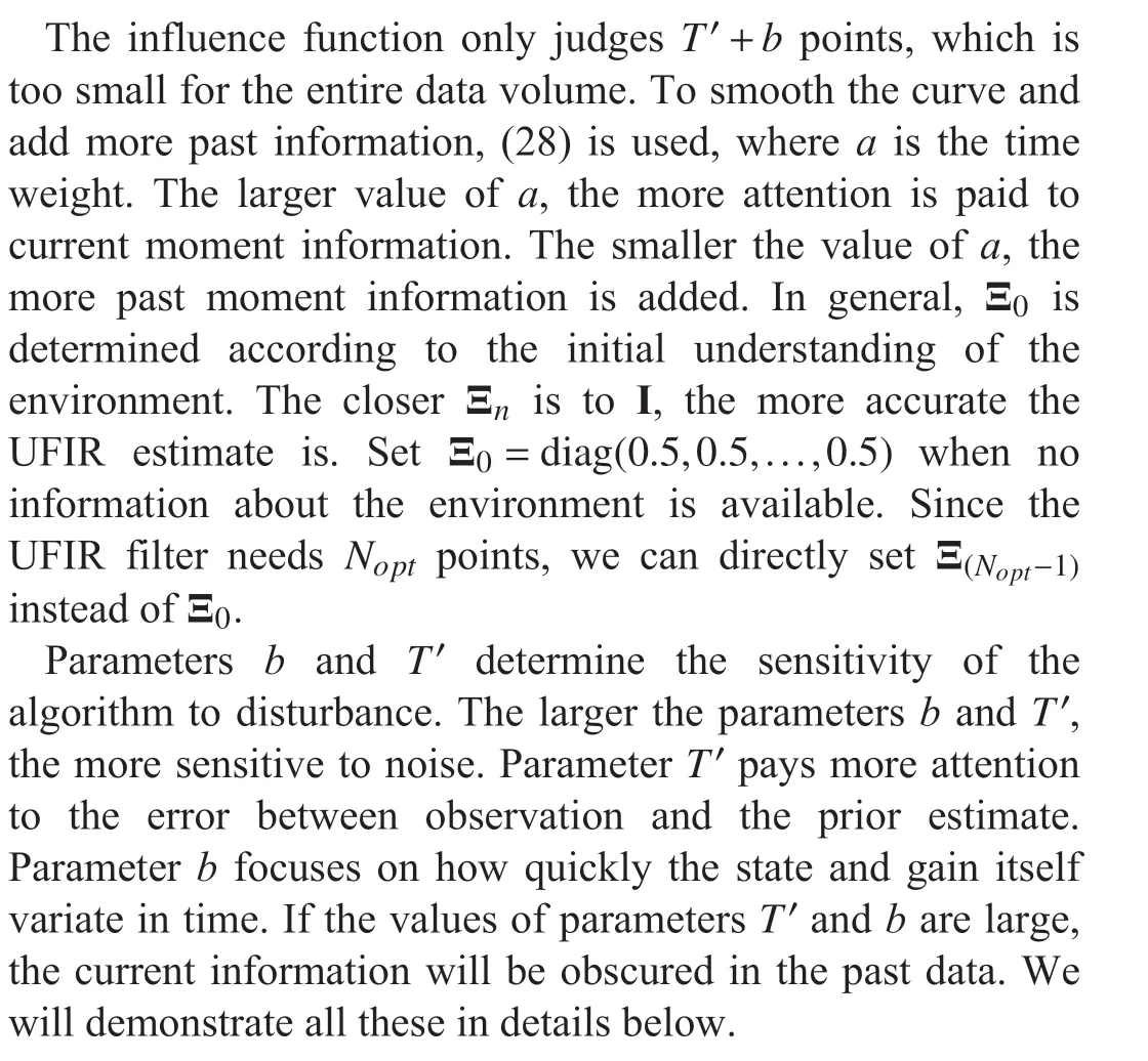
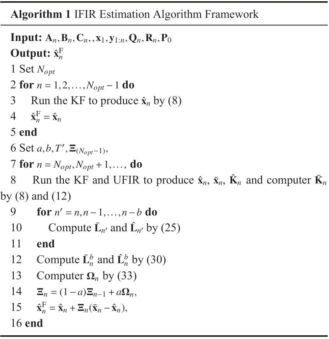
Algorithm 1 IFIR Estimation Algorithm Framework Input:An,Bn,Cn,,x1,y1:n,Qn,Rn,P0 Output:ˆxFn 1 Set Nopt 2 for do n=1,2,...,Nopt −1 3 Run the KF to produce by (8)ˆxFn = ˆxn 4 ˆxn 5 end a,b,T′,Ξ(Nopt−1),6 Set 7 for do n=Nopt,Nopt+1,...,ˆxn ¯xn ˆKn¯Kn 8 Run the KF and UFIR to produce , , and computer by (8) and (12)n′=n,n−1,...,n−b 9 for do¯Ln′ˆLn′10 Compute and by (25)11 end¯LbnˆLbn 12 Compute and by (30)13 Computer by (33)Ξn=(1−a)Ξn−1+aΩn,Ωn 14 ˆxFn = ˆxn+Ξn(¯xn −ˆxn),15 16 end
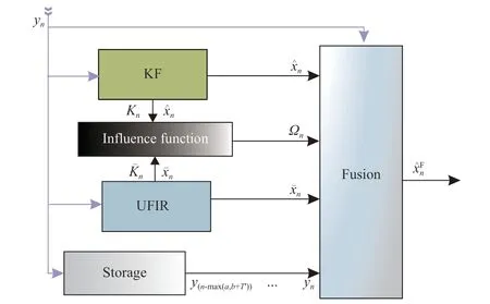
Fig. 2. A block diagram of the proposed IFIR filtering framework.
As can be seen, we only consider the diagonal elements in(33). The reason is that the proposed structure is designed for each state, and the influence between state components cannot be calculated. Specifically, the method determines the fusion relationship between the prior state estimate and the residual,and it is not suitable to use this residual to correct between states.
IV. APPLICATIONS
In this section, we demonstrate the effectiveness of the proposed approach (Algorithm 1, denoted as IFIR) by comparing it with the UFIR filter [15], the KF, and the fusion method (fusion FIR filter, denoted as fusion filter (FF) in this section) proposed in [27]. The root mean square errors(RMSEs) and the cumulative error of different algorithms are used as the main performance indicators. The main purpose is to provide users with a clear picture of the proposed algorithm.
A. Two-State Polynomial Model
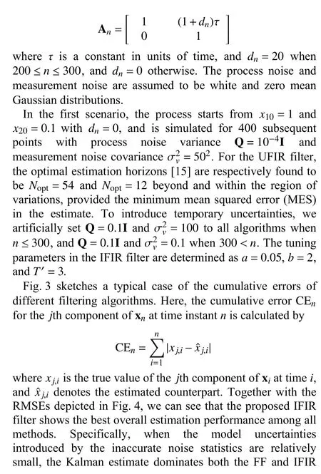
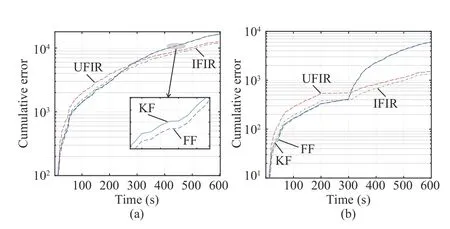
Fig. 3. Cumulative errors of different algorithms for the two-state polynomial model: (a) the first state and (b) the second state.
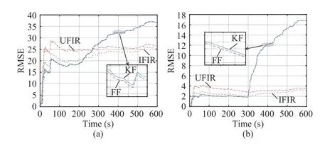
Fig. 4. RMSEs provided by different algorithms for the two-state polynomial model: (a) the first state and (b) the second state.
In this section, we apply different filtering algorithms to the two-state polynomial model (1) and (2), specified with Bn=I,Dn=I, Cn=[1,0], and algorithms, resulting in an estimation accuracy close to the KF. When modeling errors become large whenn>300, the IFIR successfully transfers its outputs to the UFIR estimates,independent of the noise covariances, while the FF method fails.
To give a clearer picture about the fusion process in the IFIR method, in Fig. 5 we show the influence values of each sub-filter in comparison with the weights of the UFIR estimates used for outputs, where the bars represent the influence values and the solid grey line represents the weights.As shown, the weight of the UFIR estimates increases along with the influence value, which can be considered a measure to quantify the effects of uncertainties on a specific filter. The filter with a significant influence values indicates that this filter is sensitive to noisy measurements and hardly matches observations.
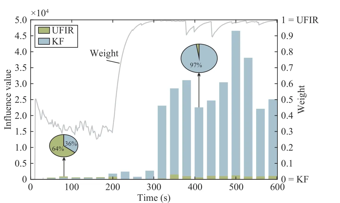
Fig. 5. In the second state, the relationship between the influence value and the weights used during filtering in the proposed algorithm.
In additions, the fusion process also illustrates another advantage of the proposed method. It is known that improvement can be achieved if we can get the error covariance at a particular moment. Using the influence function method, we can get an alternative measure of estimation covariance even if the corresponding noise statistics are unavailable.
To increase persuasiveness, we used the Monte Carlo method in the conditions of Experiment 1 to obtain Fig. 6,where the variables are random noise. As shown in Fig. 6, our proposed method has the slightest cumulative error and the best filtering effect in most cases in this experiment. Even with small probabilities, the performance of our proposed method is not the worst.
To be more illustrative, we varied only the number of experiments under the experimental conditions in Fig. 6 to obtain Table I. It can be seen that our proposed IFIR is valid under these experimental conditions.
Fig. 7 and Fig. 8 show how the values ofaandbaffect the results. As seen from the graphs, whena=0, the filter weights are constant at the initial value. There is a significant increase ata=0 in the graph, indicating that our algorithm is effective and has a much smaller RMSE than when no fusion strategy (a=0) is adopted. Fora, it can be seen that the influence values are sensitive to random disturbances, andthe same regularity exists between historical and current information. Values ofbabove a certain range will not impact the effectiveness of the filter. However, when the noise covariance is time-varying, andbexceeds a certain value and then increases, it makes the IFIR filter significantly less effective. This demonstrates that we have selected too much historical information in the event of a change in the environment, making the influence values less sensitive to the current environment.

TABLE I n TRIALS IFIR WITH MINIMUM PROBABILITY OF CUMULATIVE ERRORS
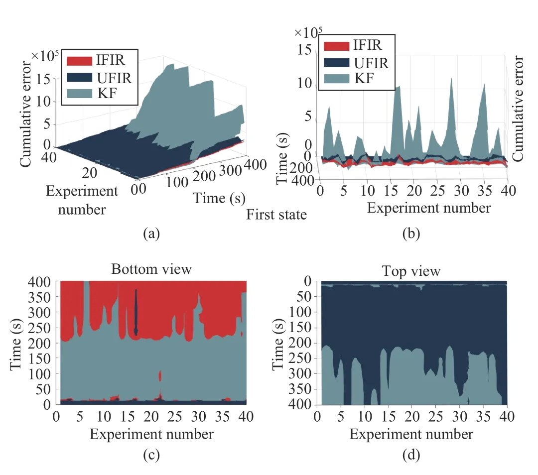
Fig. 6. Cumulative error of multiple simulations (Section IV-A): (a) Side view; (b) Front view; (c) Bottom view; and (d) Top view.
B. Quadruple Water Tank System
In this section, we verify the observations using a quadruple water tank system [37]. As can be seen from Fig. 9, two pumps feed water into different tanks using two split flows,and Tank 3 and Tank 4 also feed water into Tank 1 and Tank 2,respectively. The water in the upper tank can only be discharged into the tank below it, and the water discharged from the bottom of the tank flows directly into the large reservoir. By using the voltages applied to the two pumps as inputs and defining the system state vector as those small uncertainties in the system have a large response in the influence values. Therefore a small value ofais appropriate. A too-large value ofawould cause the IFIR weights to jump back and forth between 0 and 1, causing the random nature of the noise to mask its regular component. Forb, it shows that when the noise covariance is time-invariant,

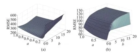
Fig. 7. RMSEs computed as functions of a and b in the presence of timevariant process noise covariances: (a) the first state, and (b) the second state.
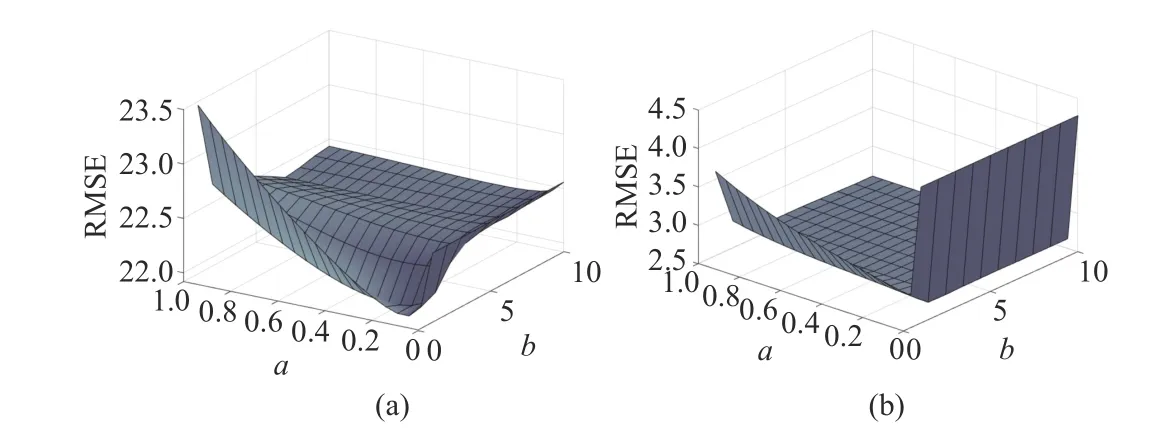
Fig. 8. RMSEs computed as functions of a and b in the presence of timeinvariant process noise covariances: (a) the first state, and (b) the second state.
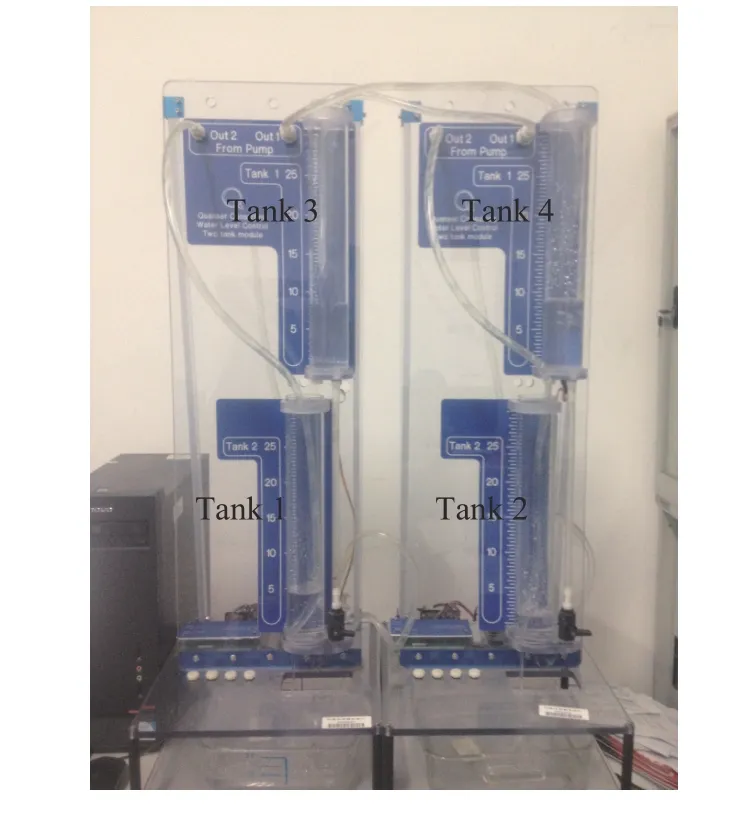
Fig. 9. The quadruple water tank system.
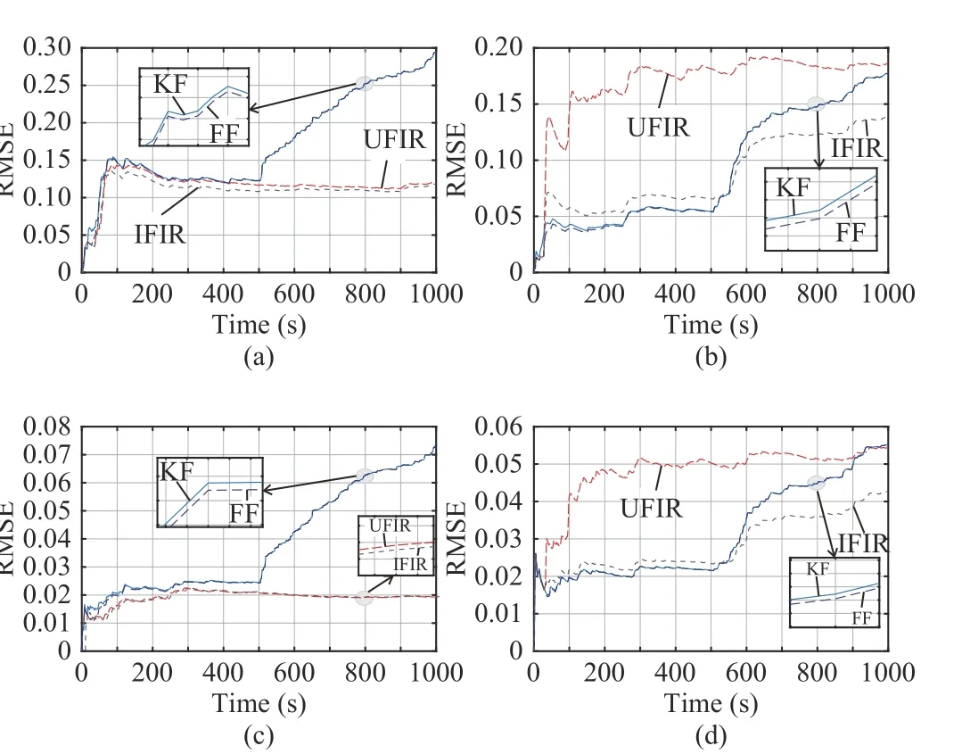
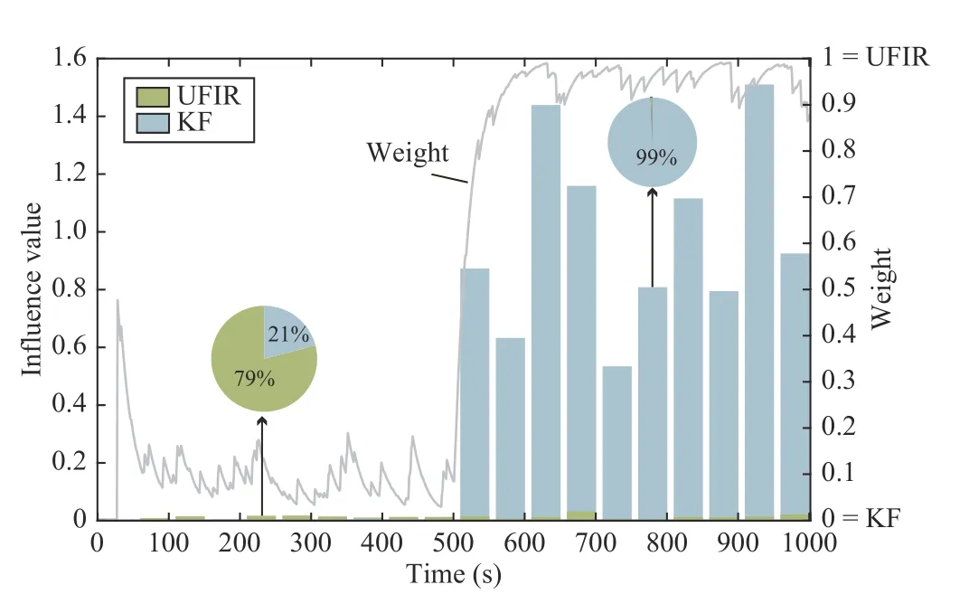
In this scenario, we generate the process at 1000 points starting with x0=[0 0 0 0]T. For the UFIR filter, the optimal estimation horizon [37] is found to beNopt=29. To introduce temporary uncertainties, we artificially set Qn=10−2I and Rn=[6 1;1 10]to all the algorithms whenn≤500, and Qn=Iand Rn=[6 1;1 10] when 500 Fig. 10 sketches a typical case of the cumulative errors of different filtering algorithms. Here, the cumulative errorCEnis the same as defined in A. Together with the RMSEs depicted in Fig. 11, we can see that the proposed IFIR filter shows the best overall estimation performance among all the methods. Specifically, when model uncertainty introduced by inaccurate noise statistics is relatively small, Kalman estimation dominates both the FF and IFIR algorithms,leading to estimation accuracy close to the KF. When model errors become large, IFIR successfully shifts its output to UFIR estimates independent of the noise covariance, while the FF approach fails. In summary, IFIR filters can determine the effectiveness of the KF and UFIR filters and fuse them based on this and synchronously follow the more effective filter as its time changes. Fig. 10. Cumulative error provided by different algorithms for the quadruple water tank system: (a) the first state, (b) the second state, (c) the third state, and (d) the fourth state. To give a clearer picture of the fusion process in the IFIR method, in Fig. 12 we show the influence values of each subfilter in comparison with the weights of the UFIR estimates used for outputs, where the bars represent the influence values and the solid grey line represents the weights. It is worth noting that this graph is only the change in IFIR weights for state 4. The IFIR weights for each state are not the same at the same moment. This means that the IFIR filter is fused for each state, and each state does not face the same situation. Fig. 11. RMSEs provided by different algorithms for the quadruple water tank system: (a) the first state, (b) the second state, (c) the third state, and (d)the fourth state. Fig. 12. In the fourth state, the relationship between the influence value and the weights used during filtering in the proposed algorithm. A new fusion filter that uses the KF and the UFIR filter as sub-filters is proposed for the discrete-time state-space model in this paper. The IFIR inherits the advantages of the KF and the UFIR filter and can vary from the Kalman estimate to the UFIR estimate. The main advantage of the proposed method is that the error covariance matrix is not required during the fusing process. The performance of the IFIR filter is demonstrated by a two-state polynomial system and a quadruple water tank system. We have seen the great potential of influence functions and believe that they contribute to the study of online evaluation filters.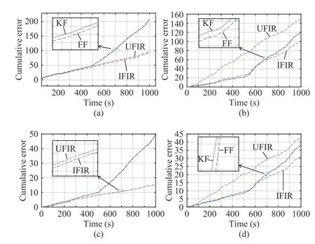
V. CONCLUSIONS
 IEEE/CAA Journal of Automatica Sinica2022年4期
- IEEE/CAA Journal of Automatica Sinica的其它文章
- Energy Theft Detection in Smart Grids: Taxonomy,Comparative Analysis, Challenges, and Future Research Directions
- On the System Performance of Mobile Edge Computing in an Uplink NOMA WSN With a Multiantenna Access Point Over Nakagami-m Fading
- Continuous-Time Prediction of Industrial Paste Thickener System With Differential ODE-Net
- Unmanned Aerial Vehicles: Control Methods and Future Challenges
- A Braille Reading System Based on Electrotactile Display With Flexible Electrode Array
- A Short-Term Precipitation Prediction Model Based on Spatiotemporal Convolution Network and Ensemble Empirical Mode Decomposition
