Detection and Attribution of Changes in Thermal Discomfort over China during 1961-2014 and Future Projections

Wanling LI, Xin HAO*,2, Li WANG, Yuqing LI, Jiandong LI, Huixin LI,2, and Tingting HAN,2

1Collaborative Innovation Center on Forecast and Evaluation of Meteorological Disasters/Key Laboratory of Meteorological Disaster, Ministry of Education, Nanjing University of Information Science and Technology, Nanjing 210044, China

2Nansen-Zhu International Research Center, Institute of Atmospheric Physics,Chinese Academy of Sciences, Beijing 100029, China

3Jiangsu Key Laboratory of Atmospheric Environment Monitoring and Pollution Control, Jiangsu Collaborative Innovation Center of Atmospheric Environment and Equipment Technology,School of Environmental Science and Engineering, Nanjing University of Information Science &,Technology, Nanjing 210044, China

ABSTRACT In this study, variation in the frequency of thermal discomfort days over China during the period of 1961-2014,including heat discomfort days (HDDs) and cold discomfort days (CDDs), and the influence of external forcings on it are discussed. HDDs are the conditions of overheating and overhumidity (represented by humidity index), and CDDs reflect the dangers from cold temperatures and winds (represented by wind chill index). Observations show significant increases(decreases) in the frequency of HDDs (CDDs) over China from 1961 to 2014, with clear regional distinctions. The historical ALL and greenhouse gas (GHG) simulations can sufficiently reproduce the spatial patterns of the observational trend in the frequency of both HDDs and CDDs over China. Further, the impacts of GHG and anthropogenic forcings on the HDDs (CDDs) are detectable over China, except for central and eastern China, based on the optimal fingerprinting method. GHG forcing is identified as a dominant factor for the observational changes in the frequency of HDDs over southern China; GHG and anthropogenic forcings have dominant effects on the variation in the frequency of CDDs over southwestern China. Although trends in the frequency of HDDs and CDDs in historical aerosol forcing simulations seems to be opposite to observations, an aerosol signal fails to be detected. Natural forcing contributes to the observational variation in the frequency of HDDs over northwestern China. In addition, the future projections of thermal discomfort days indicate that Chinese residents will face more threats of heat discomfort and fewer threats of cold discomfort in the future under global warming.

Key words: thermal discomfort, greenhouse gas, anthropogenic influence, natural forcing, aerosol forcing

1. Introduction

Outdoor comfort is important to maintaining the sustainable development of society due to its close relation to quality of life and social vitality (McMichael et al., 2006), such as outdoor activities (Chen and Ng, 2012), pedestrian traffic patterns (Hass-Klau, 1993), and disease risks (Han et al.,2020). Personal characteristics that include physiological and psychological states (age, gender, health condition, past experience, expectation, adaptation, and behavior) play critical roles in outdoor comfort (Middel et al., 2016). Microclimate conditions are other influential parameters (Piselli et al., 2018). Air temperature, humidity, and other meteorological elements change the body’s function balance via heat exchange between the human body and environment, which greatly impacts outdoor comfort (McMichael et al., 2006).

Interest in outdoor comfort has increased in recent decades. Some studies have focused on assessment methods for quantifying the level of human outdoor comfort. Various outdoor comfort indices have been proposed, especially those relating to outdoor thermal comfort (OTC), which is extremely dependent on local microclimates. Early studies provided the “effective temperature,” defined as the thermal comfort index that determined the relative effects of air temperature and humidity on thermal comfort (Houghten and Yaglou, 1923; Wu et al., 2017). Then, more accurate and universal indices, such as “physiological equivalent temperature” (Mayer and Höppe, 1987), were developed for the biometeorological assessment of the outdoor thermal environment considering the cooling effect of wind based on a thermophysiological heat-balance model. The predicted mean vote (Fanger, 1970) was proposed to predict the mean thermal response of a large population of people considering microclimatic conditions and thermal expectations.Yaglou and Minard (1957) described a “wet-bulb globe thermometer” index to investigate the heat stress of an environment defined by temperature, radiation, humidity, and wind.To evaluate the risk of freezing weather-related injuries, the“wind-chill” index was developed in Steadman (1971) and refined as the “apparent temperature” index by Steadman(1979).

OTC indices are widely applied across various regions to measure thermal perceptions under different climate conditions (e.g., Nikolopoulou and Lykoudis, 2006; Cheng et al.,2010; Pantavou et al., 2011; Lin et al., 2019). Terjung(1968) analyzed OTC and found that extreme heat stress,which occurs when the body is under stress from overheating resulting in a high risk of heat-related illnesses, appears mainly in the great low-latitude deserts of the world, and extreme heat stress is less likely in mild climates that occur near cool-current littorals and low-latitude highlands. Using four OTC indices, Pantavou et al. (2011) found that the discomfort index is closely related to the number of heataffected patients and that this number exhibited an increasing trend during the extremely hot periods during the summer of 2007 in the city of Athens, Greece. Similar situations have also been found in other regions, such as Europe and Iran, and heat waves have caused many deaths due to suffering from prolonged and serious heat stress (Beniston,2004; Roshan et al., 2018). Raymond et al. (2020) indicated that a wet-bulb temperature of 35°C, marking the upper physiological limit of humans, has already been reported in some coastal subtropical locations since 1979, and extreme wet-bulb temperatures have increased rapidly over the last four decades and will regularly exceed 35°C as a result of global warming. In contrast, cold and uncomfortable days have decreased over the past decades (Thorsson et al., 2011;Huang et al., 2020).

In China, OTC has regional characteristics, and its variability has obvious decadal fluctuations with varied turning points between regions (Wang et al., 2012; Zeng and Dong,2015; Lin et al., 2019; Wu et al., 2019). In particular,“strong hot stresses” occur in southern China, and “strong cold stresses” occur in northern China (Yue et al., 2019).Although an increasing trend in mild weather has recently occurred in China during summer, spring, and autumn,uncomfortable days have also shown an upward trend over the past few decades, which suggests stronger outdoor heat stresses in southern China and weaker outdoor cold stresses in northern China (Zhang, 2014; Kong et al., 2016; Lin et al., 2019; Wu et al., 2019). Based on the effective temperature, decreases of cold days and increases of hot days were found over China in winter and summer, respectively,which can be attributed to an increase of temperature and a decrease of wind speed (Wu et al., 2017).

Global warming exposes people to increasingly atypical weather conditions relative to preindustrial conditions(Moore et al., 2019), such as higher average air temperatures (Hansen and Lebedeff, 1987), more frequent and extreme heat waves (Russo et al., 2019; Perkins-Kirkpatrick and Lewis, 2020), and significantly changed moisture levels (Chou et al., 2009). These changing conditions are closely connected to human thermal comfort, which cannot be explained without anthropogenic effects (Bindoff et al., 2013; Sarojini et al., 2016; Gao et al., 2018). However, a majority of studies on the influence of anthropogenic activity on OTC have focused on the role of urban greening(Bowler et al., 2010), and yet its influence remains unclear.Given the regional distinction of climate, this study aims to explore this research gap over China and its sub-regions as follows: (1) updating historical changes in the frequency of outdoor thermal discomfort days during 1961-2014;(2) detecting the influence of different external forcings on the historical changes based on the optimal fingerprinting method; (3) projecting the future changes in the frequency of outdoor thermal discomfort days under different shared socioeconomic pathway scenarios. The results can provide detailed and valuable information on climate change adaptation to policy makers.

2. Materials and methods

2.1. Data

The gridded daily observation dataset used in this study, including surface wind, surface air temperature, and relative humidity parameters during the period of 1961-2014,is obtained from CN05.1 (Wu and Gao, 2013). The CN05.1 dataset, which has a horizontal resolution of 0.25° × 0.25°,was constructed by interpolation of data from more than 2400 stations across China using the “anomaly approach”method (Xu et al., 2009).

For detection and attribution of the thermal discomfort across China, the daily dataset during 1961-2014 from the Coupled Model Intercomparison Project Phase 6 (CMIP6;Eyring et al., 2016) was used, including historical all (ALL)forcing experiments (anthropogenic and natural forcing), historical natural (NAT) forcing experiments, historical greenhouse gas (GHG) forcing experiments, and historical anthropogenic aerosol (AER) forcing experiments. Additionally,54 chunks of nonoverlapping 54-year data from preindustrial nonforced control experiments (pi-control; 2916 years in total) were used for detection and attribution. Also, simulations under shared socioeconomic pathway scenarios(SSP1-2.6, SSP2-4.5, SPP3-7.0, and SSP5-8.5; O’Neill et al., 2014) from the CMIP6 models were used to project the future changes in the frequency of thermal discomfort days over China. In this study, six CMIP6 models are selected for which daily surface wind, surface air temperature, and relative humidity data are available (Table 1). Here, to give equivalent weight to each model, the ensemble means of each model are obtained and represent the simulation result.

2.2. Methods

2.2.1. OTC indices

Temperature is the main meteorological factor affecting human comfort, followed by relative humidity and wind velocity (Steadman, 1979; Mayer and Hӧppe, 1987; Stathopoulos et al., 2004). In this study, the humidity index (Humidex), defined by temperature and humidity, was used to analyze heat discomfort in China. Humidex quantifies the dangers from overheating and overhumidity with little to no discomfort, some discomfort, great discomfort, and heat stroke likely. The wind chill index (WCI), affected by temperature, humidity, and wind, was selected to analyze cold discomfort in China. These two indices have been commonly used in previous studies (Osczevski and Bluestein, 2005;Stathopoulos, 2006).

Humidex is an index that considers the comprehensive influence of temperature and humidity, which can reflect the discomfort of the human body under the conditions of overheating and overhumidity. It can be calculated as follows (Mekis et al., 2015):

where T is the temperature at a height of 2 m (units: °C) and Tdewis the dew point temperature (units: °C). The constant of 5417.753 is determined by the water molecular weight, latent heat of evaporation, and gas constant, and 273.16 represents the Kelvin ice melting point. When Humidex exceeds 30, the environmental conditions make people feel less comfortable, and outdoor activities should be appropriately reduced according to age and physical condition. When Humidex exceeds 40, people feel extremely uncomfortable, and unnecessary outdoor activities should be completely eliminated. In this study, the threshold ofH≥40 was determined as the indicator of the frequency of heat discomfort days(HDDs; Table S1 in the Electronic Supplementary Materials, ESM).

Table 1. List of information for the different experiments.

The WCI represents the human perception of cold discomfort caused by reductions in body temperature, which reflects the flow of low-temperature air and the loss of heat on the human skin surface through conduction, evaporation,convection, and radiation. The WCI is calculated by surface temperature and wind at a height of 10 m (Mekis et al.,2015). When the temperature is below zero, there are two different formulas: one for low wind speeds and one for high wind speeds. For low wind speeds (V10m＜1.39ms-1), the formula is as follows:

For high wind speeds (V10m≥1.39ms-1), the formula is as follows:

where T is the air temperature at a height of 2 m andV10mis the wind at a height of 10 m. According to the grade standard of the WCI (Mekis et al.，2015), the threshold of the fre-quency of cold discomfort days (CDDs) is set to WCI ≤-30.

2.2.2. Iterative method to calculate dew point temperature

In this paper, the dew point temperature (Tdew) is used to calculate Humidex, but there is no such meteorological element in the observational dataset. We applied an iterative method to calculate Tdew. This means that with a constant water vapor content, Tdewcan be obtained when the air mass reaches saturation through continuous cooling. The iterative method for Tdewis a mathematical method that involves the following:

(1) The saturated vapor pressure esis calculated at the current temperature as es=6.1078exp[a(T-273.16)/(T-b)];

(2) The vapor pressure is calculated at the current temperature as e =esRH/100;

(3) As the basis for judgment, e is the unchanged value here;

(4) In the case of e＜es, the temperature is continuously reduced by 0.05°C, and esis calculated until e=es,i.e., when Tdewequals T.

Here, RH and T represent the relative humidity (units:%) and air temperature at a height of 2 m (units: K), respectively. a and b are constants that involve the following:

(3) when - 15°C＞T＞-40°C, a and b can be obtained through linear interpolation analysis.

2.2.3. Optimal fingerprinting method

In this study, we applied the optimal fingerprinting method to detect and attribute changes in the frequency of thermal (heat or cold) discomfort over China from 1961 to 2014 using observations and simulations. Essentially, this method is based on the concept of the least squares method,which can be described by the following regression equation (Ribes et al., 2013):

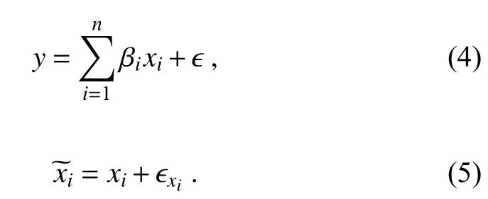
In Eq. (4), y is observed uncomfortable days, and xiis the response of the frequency of thermal discomfort days to the ith external forcing simulated by the CMIP6 models,including the NAT forcing, GHG forcing, AER forcing, and anthropogenic (ANT) forcing experiments. Here, the ANT impact was obtained as ALL minus NAT (Zhang et al.,2013), and the impact of anthropogenic activities, such as land use, was obtained by ANT minus GHG+AER (Li et al.,2017). βiis the scaling factor that adjusts the fingerprint value to produce the best match for the observations, and n represents the number of external forcing factors considered. To obtain a more accurate attribution analysis of changes in the frequency of thermal discomfort days, such changes under a single factor (the n value is one) and multiple factors (the n value is greater than one) are considered separately. ϵ represents the internal climate variability factor, which is the Gaussian distribution random residual term. The control experiments (CTL) contain 54 segments of 54-year nonoverlapping uncomfortable day datasets simulated in pi-control experiments. To avoid spurious detections, half of these segments were used to calculate the 5%-95% uncertainty of the regression coefficients related to the scaling factor β by regressing the observational frequency of thermal discomfort onto the simulated frequency of thermal discomfort based on the multimodel ensemble median (MME) of ALL, GHG, NAT, AER, and ANT, and the other half segments were used to prewhiten the data. It is worth noting that all variables in the input dataset are anomalies of the original data. To test the residual items, we used the method proposed by Allen and Stott (2003) to carry out a residual consistency test, as shown in Eq. (5). xiis assumed to be an unknown quantity, and ϵxiconsists of random items based on the MME related to the internal variability.

Using the optimal fingerprinting method, the 5%-95%margin of βiis a key indicator for estimating the consistency between the climatic response to different external forcings and observations and further investigating the attributable change in the frequency of thermal discomfort days over China by internal variation or external forcing. The 5%-95% marginal of βiis greater than zero, which means that the attributable change in the frequency of thermal discomfort days by the ith external forcing is consistent with the observations (signals of trends are the same), and the impact of the ith external forcing can be detected. The 5%-95% marginal of βiincludes one, which means that the magnitude of the impact of the i th external forcing is consistent with the magnitude of the change in observations. The 5%-95% margin of βiis greater than zero and includes one,which means that the impact of the ith external forcing passes the consistency test. More detailed information can be found in Allen and Stott (2003).

3. Results and discussion

3.1. Performance evaluations in the simulation of HDDs and CDDs

The capacity of CMIP6 models in reproducing historical climatology and linear trends of the frequency of thermal discomfort days is evaluated before detection and attribution. Figures 1a and 2a show the observational climatology and linear trends of the frequency of HDDs over China over the period of 1961-2014 based on CN05.1. As seen in Fig. 1a, the greatest frequency of HDDs occurred over southern China, followed by eastern China. Pronounced increases were observed in the frequency of HDDs over northern and southern China from 1961 to 2014 (Fig. 2a). On the other hand, CDDs mainly occurred in northern and northwestern China (Fig. 1c), and the frequency of CDDs decreased in these regions from 1961 to 2014 (Fig. 2c). These results are consistent with previous studies (e.g., Yue et al., 2019). Due to the regional characteristics of thermal discomfort days over China, we divided China territory into eight subregions to study thermal discomfort (Fig. 1a), including Northwest China (NWC), North China (NC), Northeast China(NEC), Southwest China part1 (SWC1), Central China(CC), Eastern China (EC), Southwest China part2 (SWC2),and South China (SC). These sub-regions have been widely used in climate change studies over China (e.g., Zhou et al.,2016; Wu et al., 2017).

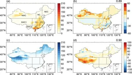
Fig. 1. Climatology (units: d) of the frequency of (a) HDDs and (c) CDDs during 1961-2014 based on CN05.1, and differences (units: d) in the frequency of (b) HDDs and (d) CDDs between the MME of historical simulations from six CMIP6 models and observations. The eight sub-regions over China are shown in (a), including Northwest China(NWC), North China (NC), Northeast China (NEC), Southwest China part1 (SWC1), Central China (CC), Eastern China (EC), Southwest China part2 (SWC2), and South China (SC). The numerical values in the top right corner of panels are the spatial correlations between observations and simulations.

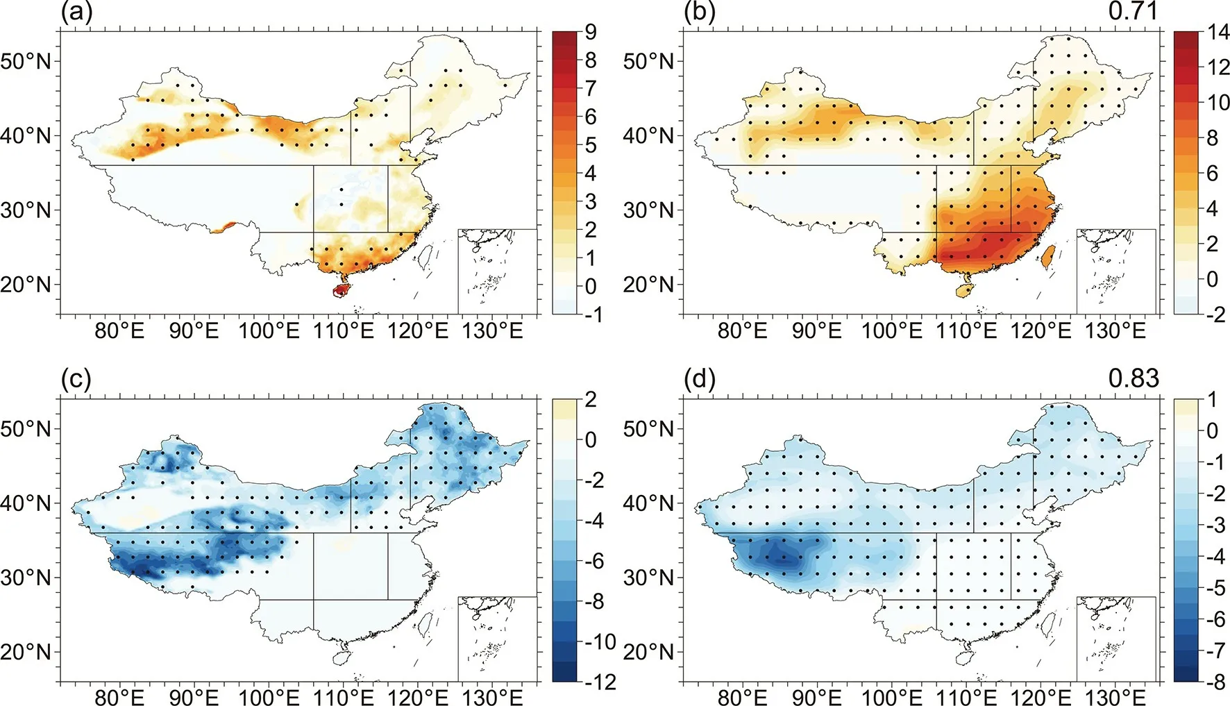
Fig. 2. Linear trends [units: d (10 yr)-1] in the frequency of HDDs (upper row) and CDDs (lower row) for (a, c)observations based on CN05.1 and (b, d) the MME of historical simulations from six CMIP6 models from 1961 to 2014. The numerical values in the top right corner of panels are the spatial correlations between observations and simulations. The dotted area indicates that the linear trend is significant at the 95% confidence level.

The spatial correlations of the climatology between individual models and observations are all greater than 0.75,and the spatial correlations of the climatology between the MME and observations reach 0.89 for HDDs and 0.90 for CDDs. This suggests that the climatology of the frequency of HDDs and CDDs in the historical simulations resembles the observations. In the individual historical simulations and the MME, more HDDs were found in southern and eastern China (Figs. 1b and S1 in the ESM), while CDDs mostly occurred in northern and northwestern China during 1961-2014 (Figs. 1d and S2 in the ESM). However, there are biases in the climatology between observations and simulations (Figs. 1b, 1d, and S1-2 in the ESM). For example,the MME greatly overestimates the frequency of HDDs in NWC and the frequency of CDDs in SWC1.

The linear trend of the frequency of HDDs and CDDs from 1961 to 2014 in the models are shown in Figs. 2b, 2d,S3, and S4 in the ESM. Similar to observations, there were significant increases in the frequency of HDDs over NWC,NC, NEC, and SC for the MME and individual models(except for GFDL-ESM4; Figs. 2b and S3). Meanwhile, an increase in the frequency of HDDs also was found over CC and EC in both the MME and individual models, which was not observed in observations. For the frequency of CDDs,the MME and individual historical simulations reproduce the observational decreases over China well, except for GFDL-ESM4 (Figs. 2d and S4). The spatial correlations of linear trend in the frequency of HDDs (CDDs) between individual models (CanESM5, HadGEM3-GC31-LL, MRIESM2-0, IPSL-CM6A-LR, and MIROC6) and observations are greater than 0.57 (0.73), and the spatial correlation of linear trend in the MME and observations reaches 0.71(0.83). Results show that historical linear trends in the frequency of HDDs and CDDs from these five models and the MME present a good resemblance to observations. In general, five CMIP6 models (CanESM5, HadGEM3-GC31-LL,MRI-ESM2-0, IPSL-CM6A-LR, and MIROC6) could simultaneously reproduce the climatology and trends of the frequency of HDDs and CDDs over China sufficiently; thus,these five models were chosen for further analyses.

Furthermore, time series of regional mean frequency of HDDs and CDDs anomalies from 1961 to 2014 are shown in Figs. S5 and S6 in the ESM. It is obvious that the historical frequency of HDDs and CDDs over the eight subregions shows remarkable interannual-to-decadal changes,as well as long-term trend. Many studies have suggested that the western Pacific subtropical high plays an important role in decadal variations of hot days over eastern China and the eastward shift of the western Pacific subtropical high has caused less hot days over eastern China since the mid-1970s (Ding and Chan, 2005; Huang et al., 2015;Wang et al., 2016; Liu et al., 2019). The results of these studies agree well with the decadal changes in the historical frequency of HDDs over CC and EC (Fig. S5 in the ESM).The long-term decrease and interdecadal oscillation in the historical frequency of CDDs over NWC, NC, and NEC may be linked to the weakening and interdecadal variations of the East Asian winter monsoon (Ding et al., 2014; Hao et al., 2019). In the MME of historical simulations, the trend value is close to the observational value in NWC, NC, NEC,SWC1, SWC2, and SC (Figs. S5 and S6 in the ESM).However, false trends in the frequency of HDDs and CDDs from 1961 to 2014 simulated by the MME over EC and CC may be a barrier to the following attribution and future projection.

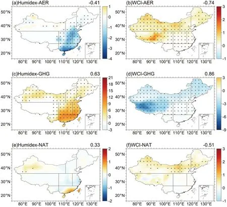
Fig. 3. Linear trends [unit: d (10 yr)-1] in the frequency of HDDs (left column) and CDDs (right column) for (a, b)AER forcing, (c, d) GHG forcing, and (e, f) NAT forcing from 1961 to 2014. The results from the MME of the five chosen models are shown. The numerical values in the top right corner of panels are the spatial correlations between observations and simulations. The dotted area indicates that the linear trend is significant at the 95% confidence level.

3.2. Detection and attribution of thermal discomfort in China

Historical experiments reveal the combined effects of natural forcing and anthropogenic forcing (e.g., greenhouse gas, aerosol, land use), and it is difficult to understand their individual roles in the thermal discomfort over China. We conduct an analysis on the individual role of each factor in thermal discomfort.

Figure 3 shows the linear trend in the response of the frequency of thermal discomfort days to historical AER, GHG,and NAT forcings during the period of 1961-2014. The linear trends forced by AER are opposite to those forced by ALL but have similar spatial distribution (Figs. 3a-b and S7 in the ESM). Under AER forcing, the frequency of HDDs shows a significant reduction over CC, EC, and SC in the MME and individual models, which may be attributed to the AER-induced cooling over southeastern China through aerosol-radiation interaction in summer. The frequency of CDDs exhibits an increase in NWC, NC, NEC, and SWC1,which may result from the warming over northern China through cloud feedbacks related to aerosol-induced cooling over the tropical Indian Ocean and western tropical Pacific in winter (Chen and Dong, 2019). Obviously, large diversity exists in the effect of AER forcing on the long-term trend of the frequency of HDDs over NWC, NC, and EC, as well as the frequency of CDDs over NEC, CC, EC, and SC. The results based on the GHG forcing show that the linear trends in the frequency of HDDs and CDDs are extremely similar to the results of the ALL forcing. It shows a significant increase in the frequency of HDDs over China except for SWC1 and a decrease in the frequency of CDDs over the cold areas (NEC, NC, NWC, and SWC1; Figs. 3c-d and S8 in the ESM). The spatial correlations of linear trends in the frequency of HDDs (CDDs) between the GHG forcing and observations are all greater than 0.51 (0.66), and the spatial correlation between the MME and observations reaches 0.63 (0.86). This indicates that there is a remarkable resemblance between the results based on the GHG forcing and observations in terms of the trends in the frequency of HDDs and CDDs. Unlike the AER and GHG forcings, four out of five models display no obvious trend change in the frequency of HDDs and CDDs over most regions of China under the NAT forcing (Figs. 3e-f and S9 in the ESM).Only in the MME and MIROC6 do the results based on the NAT forcing show extensive increases in the frequency of CDDs over NWC, NC, and NEC, which is opposite to observations. This means that the possible effects of different external forcings on thermal discomfort in China have sharp distinctions.

Furthermore, we conducted a quantitative analysis to investigate the extent to which these external forcings can exert influences on the variations of thermal discomfort days over China and within its sub-regions, using the optimal fingerprinting method. According to one-signal analyses implementing the optimal fingerprinting method, the different signals, which represent the regression coefficients of the regional mean frequency of HDDs (CDDs) in the observational dataset regressed onto the regional mean frequency in the MME with individual external forcings (ALL, GHG,AER, ANT, and NAT), should be detected. To separate the contribution of individual forcings from the combined effect, multisignal analyses were also carried out, including three-signal (AER+GHG+NAT) combinations and two-signal (ANT+NAT) combinations. Results show that the p values for all regression models are significant at the 90% confidence level based on the residual consistency test, suggesting the reliability of the scaling factors.

The detection results for the variation of the frequency of HDDs in China are shown in Fig. 4. In NWC, the 90%uncertainty ranges of the scaling factors for the ALL, GHG,NAT, and ANT forcings from both one-signal and multisignal analyses are all greater than zero, suggesting that the effects of these external forcings on the frequency of HDDs are detectable (Fig. 4a). Best estimates for the ALL forcing are close to unity, indicating it has a good resemblance to the observational variation of the frequency of HDDs. The NAT forcing can be detected (Fig. 4), but there is no trend in the responses to the NAT forcing (Fig. 3e), implying that the NAT forcing contributes to the variations of the frequency of HDDs on interannual-to-decadal time scales in NWC. In NC and SWC1, the signals of the ALL, GHG, and ANT forcings can be detected according to the above principles (Figs. 4b and 4d). The NAT forcing can only be detected in two-signal analysis, emphasizing the synergistic effect of the NAT and ANT forcings on the frequency of HDDs in NC and SWC1 (Figs. 4b and 4d). The signals of the ALL and ANT forcings are detectable, while the effect of the GHG forcing on the frequency of HDDs can only be detected in one-signal analysis over NEC (Fig. 4c). The effect of the NAT forcing is not detectable over NEC (Fig. 4c).Over CC and EC, none of the external forcings can be detected in the variations of the frequency of HDDs, except for the effect of the AER and GHG forcings in three-signal analysis (Figs. 4e-f). Similar results can be found in the results of the ALL forcing. This may be linked to the poor reproducibility of observed variation in the MME and the contribution of internal variability (Chen and Zhou, 2018; Hao et al.,2019). Over SWC2 and SC, the signals of the ALL, GHG,and ANT forcings are all detectable, and the GHG forcing is the dominant factor for the change in the frequency of HDDs; the NAT forcing is not detected (Figs. 4g and 4h). It should be noted that the effect of the AER forcing on the variation of HDDs fails to be detected in all eight sub-regions.Although the spatial linear trend signal of the AER forcing is opposite as an individual forcing factor, the scaling factor of the AER forcing in three-signal combinations is opposite,which suggests great uncertainty around its impact (Fig. 4h).

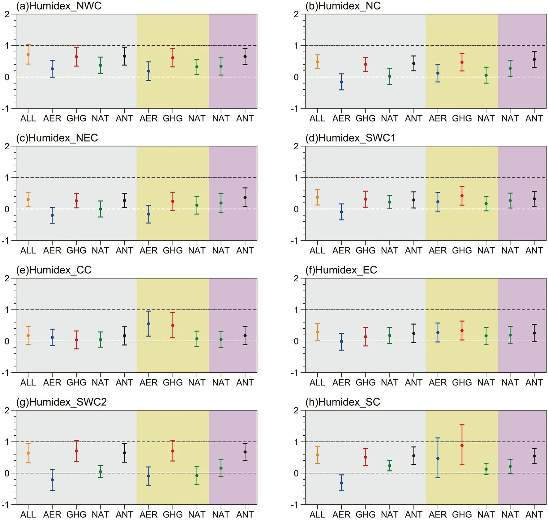
Fig. 4. Best estimates of the scaling factors from single-signal optimal fingerprinting analyses (grey shading), threesignal analyses (yellow shading), and two-signal analyses (purple shading) for the frequency of HDDs over eight sub-regions during the period 1961-2014. Error bars in subplots indicate the 5%-95% uncertainty ranges of the scaling factor. The two dashed horizontal black lines represent “0” and “1” values of the y-axis in the subplots.

Figure 5 shows the fingerprints of CDDs variations in response to external forcings. The effects of the ALL, GHG,and ANT forcings on the variation of the frequency of CDDs are detectable in NWC, NC, NEC, and SWC1; in particular, the GHG and ANT forcings have leading effects in SWC1 (Figs. 5a-d). The AER forcing can be detected in the individual regression model over NWC and SWC1, and the negative scaling factors of the AER forcing indicate an opposite effect on the variations in the frequency of CDDs (Figs. 5a and 5d). However, the NAT forcing fails to be detected over NWC, NC, NEC, and SWC1 (Figs. 5a-d). Over CC and EC, none of these external forcings are detectable, except for the effect of the ANT forcing in one-signal analysis, as well as the ALL forcing (Figs. 5e-f). This suggests that the variation of the frequency of CDDs under the ALL forcing does not resemble observations; thus, all regression models in CC and EC are invalid. It is evident that human activities,especially GHG forcing, have great influences on the frequency of CDDs in the cold areas (NWC, NC, NEC, and SWC1).

3.3. Future prediction of changes in human comfort

The above analysis shows that human activities have greatly affected the change in the frequency of HDDs and CDDs over China in the past decades. In China, with the implementation of sustainable development strategies, the future projection of thermal discomfort over China under different social and economic development scenarios is worth discussing. Figures 6 and 7 show the time series of the frequency of HDDs and CDDs in eight sub-regions during 1961-2100. Based on the MME of the selected five models,the regional mean frequency of HDDs shows an interdecadal increase, as observed in the historical period (Figs. 6 and S5). The frequency of HDDs will rapidly increase under the high-speed development and high radiative forcing scenario (SSP5-8.5) in the future. Under the scenario of local development and medium radiation forcing (SSP3-7.0), the growth rate is slower than that in SSP5-8.5. The growth rate gradually slows down under the scenario of moderate development and moderate radiative forcing (SSP2-4.5), and the frequency of HDDs will stabilize at 40-60 d yr-1in NWC (Fig. 6a), 60-80 d yr-1in NC (Fig. 6b),20-40 d yr-1in NEC (Fig. 6c), 2.5-5 d yr-1in SWC1 (Fig.6d), 75-100 d yr-1in CC (Fig. 6e), 100-125 d yr-1in EC(Fig. 6f), 25 d yr-1in SWC2 (Fig. 6g), and 150 d yr-1in SC(Fig. 6h) by the middle of the 21st century, respectively.The frequency of HDDs under the scenario of sustainable development and low radiative forcing (SSP1-2.6) shows a weak decline over China at the end of the 21st century,except for in SWC2.

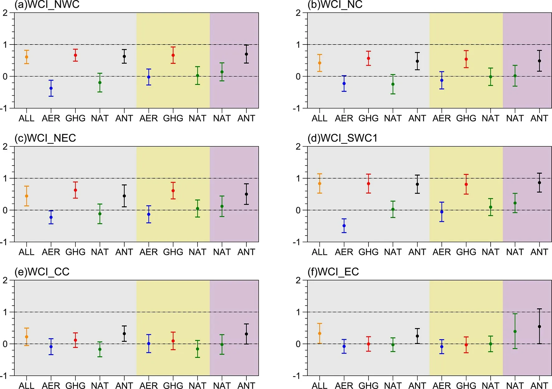
Fig. 5. Same as in Fig. 4, but for the frequency of CDDs.

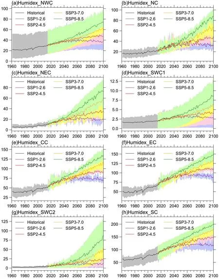
Fig. 6. Time series of the frequency of HDDs in the eight sub-regions from 1961 to 2100. The results in the historical period (black: 1961-2014) are from the historical simulations. The results in the future period (2015-2100) are the future projections under the SSP1-2.6 (purple), SSP2-4.5 (red), SSP3-7.0 (orange), and SSP5-8.5 (green) scenarios.The colored solid lines indicate the MME of the five selected models, and the corresponding shadings indicate the model spreads.

Under the SSP5-8.5 scenario, the regional mean frequency of CDDs will rapidly decrease in the future over NWC, NC, NEC, and SWC1 (Figs. 7a-d). Similar to SSP5-8.5, the results under the SSP3-7.0, SSP2-4.5, and SSP1-2.6 scenarios display a reduction but with a slower rate. At the end of the 21st century, the frequency of CDDs tends to stabilize under SSP2-4.5 and SSP1-2.6. Over CC and EC, the frequency of CDDs will drop to zero in the future (Figs. 7e-f).Moreover, it is very rare for the frequency of CDDs to to be the same for the historical and future periods over SWC2 and SC (Figs. 7g-h).

Compared with the historical period (1981-2010),except for SWC1, there are drastic increases in the frequency of HDDs over China in the future (2071-2100;Figs. 8a, 8c, 8e, and 8g). In particular, the frequency of HDDs over SC in 2071-2100 increases by more than 90 d yr-1under the SPP5-8.5 scenario, relative to 1981-2010 (Fig. 8g). Under SSP scenarios, CDDs will still occur in the cold areas (NWC, NC, NEC, and SWC1) during 2071-2100, and the largest decrease (by about 59 d yr-1) between 2071-2100 and 1981-2010 in the frequency of CDDs is found in SWC1 under the SSP5-8.5 scenario (Figs. 8b, 8d, 8f, and 8h).

Fig. 7. Same as in Fig. 6, but for the frequency of CDDs.

Fig. 8. Composite differences (units: day) in the frequency of HDDs (left column) and CDDs (right column) between the future period (2071-2100) and historical period (1981-2010). The results during 2071-2100 under the (a, b)SSP1-2.6, (c, d) SSP2-4.5, (e, f) SSP3-7.0, and (g, h) SSP5-8.5 scenarios are all shown. The dotted area indicates that the difference is significant at the 95% confidence level.

4. Conclusions

During the period of 1961-2014, HDDs occurred in NWC, NC, CC, EC, and SC; CDDs mainly occurred in NWC, NC, NEC, and SWC1. The frequency of HDDs over NWC, NC, NEC, and SC increased significantly and the frequency of CDDs over NWC, NC, NEC, and SWC1 decreased significantly during the past decades. The historical simulations performed in this study can sufficiently reproduce the spatial pattern of observational climatology and linear trends in the frequency of HDDs and CDDs over China,except for CC and EC. The GHG forcing also captures the change in the linear trends over China, while the AER forcing shows an opposite effect. Based on the optimal fingerprinting method, the ALL, GHG, and ANT forcings can be detected over China, except for CC and EC. Further, the GHG forcing is identified as the dominant factor for observational changes in the frequency of HDDs in SWC2 and SC,and GHG and ANT forcings have dominant effects on the changes in the frequency of CDDs in SWC1. The AER forcing may have a slight effect on the changes in the linear trend, but it cannot be detected in the observational changes in the frequency of both HDDs and CDDs. On the other hand, the NAT forcing contributes to the observational change in the frequency of HDDs over NWC. In the future,there will be rapid increases in the frequency of HDDs under global warming. In particular, the frequency of HDDs over SC in 2071-2100 increases by more than 90 d yr-1under the SPP5-8.5 scenario, relative to 1981-2010. The CDDs will substantially decrease in cold areas. The future projections indicate that Chinese residents will face more threats of heat discomfort and fewer threats of cold discomfort in the future under global warming.

Notably, there is diversity in the simulations of the frequency of HDDs and CDDs over China among the different models, including climatology, linear trend, and their responses to the external forcings. These biases might be limited by objective factors such as internal variability, model structural uncertainty, etc. (Giorgi and Bi, 2000; Wang and Sun, 2018). Additionally, there are also biases between the simulation and observation, which brings uncertainty to the results. The uncertainty in the results of detection and future projection is smaller in multimodel estimation than individual model estimation because of a better reproduction of the internal variability and response to external forcings(Ribes et al., 2013). In this study, only five models were used. If a large ensemble of climate models is provided and the reproducibility of the models are improved in the future,the uncertainty of the results may decrease substantially.Given the effect of outdoor thermal discomfort on human health risks, more accurate and detailed results should be sought in a future study.

Data sharing

The data that support the findings of this study are available from the authors upon request.

Acknowledgements.This work was supported by the National Natural Science Foundation of China (Grant Nos.41991283 and 42005014) and College Students’ Enterprise and Entrepreneurship Education Program of NUIST (Grant No.201910300095Y).

Electronic supplementary material:Supplementary material is available in the online version of this article at https://doi.org/10.1007/s00376-021-1168-x.