A Hybrid Neural Network Model for ENSO Prediction in Combination with Principal Oscillation Pattern Analyses

Lu ZHOU and Rong-Hua ZHANG*,3,4

1CAS Key Laboratory of Ocean Circulation and Waves, Institute of Oceanology, and Center for Ocean Mega-Science,Chinese Academy of Sciences, Qingdao 266071, China

2University of Chinese Academy of Sciences, Beijing 100029, China

3Laboratory for Ocean and Climate Dynamics, Pilot National Laboratory for Marine Science and Technology,Qingdao 266237, China

4Center for Excellence in Quaternary Science and Global Change, Chinese Academy of Sciences, Xi’an 710061, China

ABSTRACT El Niño-Southern Oscillation (ENSO) can be currently predicted reasonably well six months and longer, but large biases and uncertainties remain in its real-time prediction. Various approaches have been taken to improve understanding of ENSO processes, and different models for ENSO predictions have been developed, including linear statistical models based on principal oscillation pattern (POP) analyses, convolutional neural networks (CNNs), and so on. Here, we develop a novel hybrid model, named as POP-Net, by combining the POP analysis procedure with CNN-long short-term memory(LSTM) algorithm to predict the Niño-3.4 sea surface temperature (SST) index. ENSO predictions are compared with each other from the corresponding three models: POP model, CNN-LSTM model, and POP-Net, respectively. The POP-based pre-processing acts to enhance ENSO-related signals of interest while filtering unrelated noise. Consequently, an improved prediction is achieved in the POP-Net relative to others. The POP-Net shows a high-correlation skill for 17-month lead time prediction (correlation coefficients exceeding 0.5) during the 1994-2020 validation period. The POP-Net also alleviates the spring predictability barrier (SPB). It is concluded that value-added artificial neural networks for improved ENSO predictions are possible by including the process-oriented analyses to enhance signal representations.

Key words: ENSO prediction, the principal oscillation pattern (POP) analyses, neural network, a hybrid approach

1. Introduction

El Niño-Southern Oscillation (ENSO) is the most significant ocean-atmosphere interaction phenomenon in the equatorial Pacific Ocean, which influences the global climate system by the atmospheric bridges and oceanic pathways (Bjerknes, 1969; Zhang et al., 1998; Wang, 2019). As ENSO causes enormous natural disaster and damage worldwide; tremendous efforts have been made to develop ENSO observing systems, theories, and prediction methods over the past several decades (Cane and Zebiak, 1985; Cane et al., 1986; McCreary and Anderson, 1991; Chen et al., 1995;Philander, 1999; Mcphaden et al., 2006; Gao et al., 2018;Zhang et al., 2020; Feng et al., 2020). In particular, the advances in the observational analyses and process understanding of ENSO have led to greatly improved model developments and prediction capabilities, including dynamical and statistical models. The dynamical models can be categorized as intermediate coupled models (Hirst, 1986; Zebiak and Cane, 1987; Zhang et al., 2005; Zhang and Gao, 2016),hybrid coupled models (Barnett et al., 1993; Zhang et al.,2020) and fully coupled general circulation models (Jin et al., 2008). In addition, statistical models have been configured from historical datasets, including regression algorithms, linear and nonlinear empirical configurations.For example, principal oscillation pattern (POP; Hasselmann, 1988; Von Storch et al., 1988) analyses have been developed for extracting ENSO-related space-time evolution patterns, and corresponding POP-based statistical models have been developed for ENSO predictions (Xu, 1990).

Presently, more than 20 models have been used to make real-time ENSO predictions at lead times of 6-months and longer (see https://iri.columbia.edu/our-expertise/climate/predictions/enso/current/). Overall, current models can provide successful ENSO predictions up to six months(Latif et al., 1998; Jin et al., 2008; Barnston et al., 2012;Zhang et al., 2020; Zhang et al., 2021). However, prediction skills decline significantly beyond 6 months lead time because of the spring predictability barrier (SPB; Goddard et al., 2001; Zhang et al., 2005). Recent studies indicate that ENSO predictions are affected more strongly by SPB after the 2000s, and prediction skills from both dynamical and statistical models have declined substantially in the past 20 years (Zhang et al., 2021). This poses a great challenge for real-time ENSO prediction. To reduce biases and uncertainties in ENSO prediction, new methods are clearly needed to take advantages of new artificial intelligence (AI) techniques and improve real-time predictions.

Recently, artificial neural network (ANN) methods have emerged as a powerful approach to solving scientific problems in many areas (Abiodun et al., 2018). Briefly,ANN is a nonlinear statistical method that uses neurons to describe a function from input variables to output values. In particular, deep learning (DL) techniques have been widely applied to the geosciences in recent years (Reichstein et al.,2019; Irrgang et al., 2021). For example, this technique has been widely used for eddy identification (Xu et al., 2019),ENSO prediction (Ham et al., 2019), tropical instability wave forecasting (Zheng et al., 2020), and so on. Especially in the field of ENSO prediction, DL techniques have shown great potential for improvements. For example, Nooteboom et al. (2018) combined an autoregressive integrated moving average method with an ANN to predict the Niño-3.4 index [i.e., an area-averaged sea surface temperature(SST) anomaly in the Niño-3.4 region (5°S-5°N,170°-120°W)]. Moreover, Mu et al. (2021) designed a multivariate air-sea coupled model based on a graphical neural network for ENSO prediction. This data-driven coupled model was shown to be capable of capturing the dynamic process of ENSO evolution and to provide long-lead-time ENSO prediction. Indeed, Ham et al. (2019) formulated a convolutional neural network (CNN; LeCun and Bengio, 1995)model to predict ENSO and demonstrated that the datadriven CNN model can make skillful ENSO predictions for a lead time of 17 months. This result is systematically superior to almost all dynamical and linear statistical models.This considerable progress in ENSO prediction using ANNs gives us confidence to pursue further research and application with optimizations based on process understanding and representation of ENSO.

Note that the real coupled atmosphere-ocean system exhibits variability signals and high-frequency noise. For example, ENSO-related anomaly fields are highly spatially and temporally correlated on interannual time scales, with strong coherent space-time evolution. Various signals exist in raw observational data; some are useful for ENSO prediction, but some are not. Consequently, filtering unrelated noise from raw data before formulating ANN-based prediction models is highly desirable. Data pre-processing can be conducted in such a way that signals of interest are enhanced while unrelated noise effects are reduced. Furthermore, specific space-time evolution features of ENSO can be incorporated into the data-driven model configurations,which act to constrain prediction of ENSO-related anomalies. In earlier studies, empirical orthogonal function(EOF) analyses were used to obtain the leading principal component (PC) time series, which were then used as input for a feed-forward ANN to obtain the final outputs as prediction(Tangang et al., 1997; Wu et al., 2006). More recently, empirical mode decomposition (EMD) and ensemble empirical mode decomposition (EEMD) method have also been introduced into ANNs. Such data pre-processing reduces high dimensions of input fields (Guo et al., 2020; Yan et al.,2020; Wang et al., 2021). The addition of these pre-processing procedures led to improved prediction of ENSO using the ANN-based models. So far, there are very few studies that have accounted for space-time characteristics of ENSO (spatial patterns and quasi-periodic nature), so that three-dimensional data are appropriately treated and utilized in ANN modeling.

The focus of this study is to evaluate the efficacy of a hybrid approach by combining process-based extraction analysis methods with ANNs for long-lead predictions of ENSO. Specifically, in this paper, we develop a novel hybrid neural network model, named as POP-Net, for ENSO prediction, which is composed of the POP analyses and an ANN model (CNN-LSTM). In this hybrid configuration, the POP analysis method is first used to extract the periodically varying POP patterns and corresponding temporal coefficients from SST and oceanic heat content of the upper 300 m (T300) anomaly fields, from which the spatial features are used in the CNN-LSTM modeling; in practice, the POP analyses are added in the ANN model by a time information extraction module. Next, the POP-related temporal coefficients are combined with the feature maps generated from the CNN-LSTM model for further optimization procedure to obtain the final output as predictions.

The remainder of this paper is organized as follows: section 2 describes data, POP analysis method, detailed model configurations and prediction procedures. The validations and comparisons during the validation period between these model predictions are described in section 3. Section 4 focuses on several cases to assess prediction performances of different models, including real-time ENSO prediction for the coming year. A summary and discussion of this hybrid modeling study are given in section 5.

2. Datasets and models

2.1. Datasets

To construct various models and assess their prediction performances, various data are used. SST and T300 anomaly fields come from different datasets (Table 1). We used the Simple Ocean Data Assimilation (SODA) reanalysis products during 1871-1980 to formulate the POP model.For the ANN-based training process, we divided the predictors into pre-training and fine-training data. Because the observational period is still too short to meet the needs for having sufficiently large data, we additionally utilized data from 23 climate models during 1850-1980 that participated in the Coupled Model Intercomparison Project phase6(CMIP6; Eyring et al., 2016; details in Table 2) to preliminarily train the CNN-LSTM and the hybrid models. Nevertheless, CMIP6 models have biases, which can affect the prediction accuracy of the constructed models. So, we used the SODA reanalysis products during 1871-1980 in transfer training (Pratt et al., 1991) to further calibrate the pretrained models. Moreover, for the cross-validation analyses,the anomaly fields from Global Ocean Data Assimilation System (GODAS) reanalysis during 1994-2020 were used to evaluate prediction skills. In addition, we set an interval of more than ten years between the training and validation periods to eliminate the impact of the ocean's long-term memory on evaluation.

Table 1. Reanalysis data used in this study.

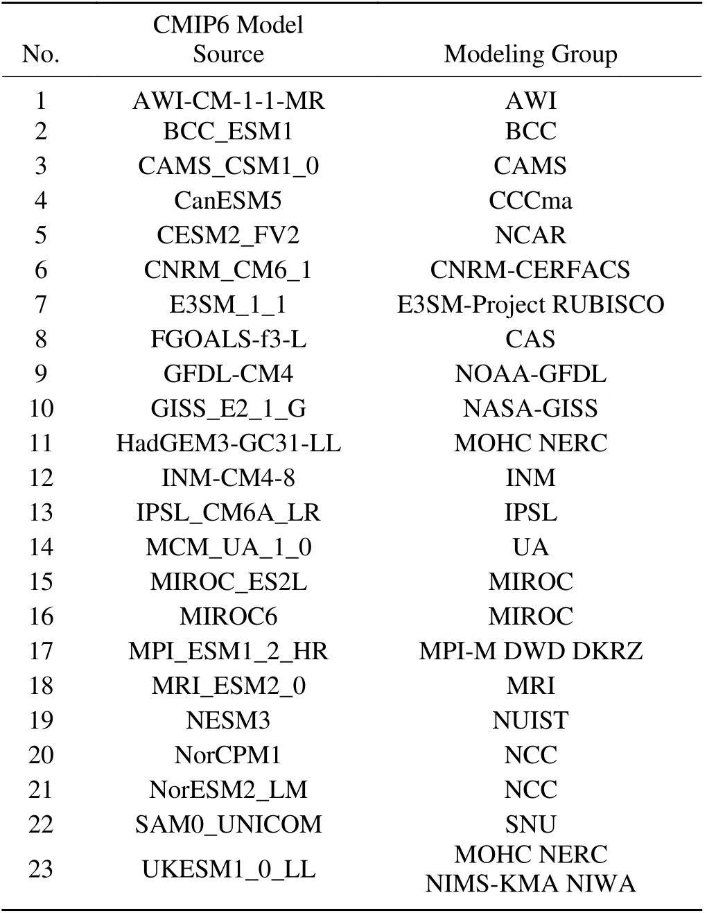
Table 2. Details of the CMIP6 models used in this study.

Table 3. Comparison among predictions made using POP, CNN-LSTM, and POP-Net models; here prediction validations are performed using GODAS dataset for 3-, 6-, 9-, and 12-month lead times. The input variables for all predictions made are SST and T300.

ENSO was quantified by using Oceanic Niño Index(ONI; i.e., three-month running mean Niño-3.4 SST index),an area-averaged SST anomaly in the Niño-3.4 region).This index is the target of the predictand in models. In predictions, the ONI value is assigned to the last month within the considered averaging window; for example, the ONI in March is assigned to the mean of the January-February-March SST index. Its purpose is to prevent the prediction models from using any data in the future.

These data were used to configure a POP-based linear statistical model, an ANN model (CNN-LSTM), and their combined hybrid model (POP-Net). Various data were further used to make comparisons among predictions from different models.

2.2. A brief overview of POP analysis method and the POP-based ENSO prediction

The climate system and its variability are too complex to be clearly isolated and analyzed using traditional statistical methods. The POP analysis method was then developed to adequately extract periodically propagating or standing patterns from a multi-component system (Von Storch et al.,1988). In this section, we describe the POP approach briefly; more details can be found in Hasselmann (1988)and Von Storch et al. (1988).

Traditionally, EOF analyses are used to yield an optimal representation of anomaly covariance matrix to compress data freedom. The POP analyses are based on EOF analyses to further extract dominant oscillation patterns.

Assuming the m-dimensional vector series composed of EOF-derived PCs is X(t), X(t) can be generated by a firstorder multivariate Markov process:

Here, t is time and ξ is Gaussian white noise matrix, which is uncorrelated with X(t). Then constant matrix B can be obtained with lag-1 and lag-0 covariance matrices of X(t).The linear system's normal modes, called POPs[Pk(k=1, 2, …,m); k is mode index], are the eigenvectors of the matrix B, which are usually complex due to the asymmetric nature of B.

In addition, the state vector X(t) can be uniquely represented in terms of eigenvectors:

where Zk(t) is the temporal coefficient of normal mode Pkat time t . In the following, for brevity, we take the complex POP modes that are often used to describe propagating features in space as examples for analyses.

When a complex POP mode pair is selected, the linear system X(t) can be reduced to a two-dimensional space spanned by the real and imaginary parts of the POP mode.Here,(t) is defined as the part of system X(t) represented by the kth pair of POPs ( Pk=Pr,k+iPi,k; i is a symbol representing the complex Pkconsisting of its real and imaginary parts), and the corresponding temporal coefficients Zk(t)[Zk(t)=Zr,k(t)+iZi,k(t)] . Thus,(t) is written as

In general, the POP analyses provide a statistical technique to extract periodic oscillation patterns in a subspace spanned by POP modes ( Pk). The corresponding temporal coefficients, Zk(t), are the coordinates in this space, representing the state of POPs. In particular, the evolution of the POPs state is explicitly specified as a dynamical model defined in Eq. (1). This linear assumption and the oscillation evolution characteristics of modes are demonstrated reasonably for ENSO research (Xu, 1990). This is the main difference between the POP analyses and any other EOF technique, which maximizes variances from a simultaneous covariance matrix. According to the scientific problems studied, the POPs with particular periods can be selected for analyses. As will be seen below in the next section, we selected two ENSO-related POPs with periods of 2-7 years for analyses and predictions.

2.2.1. Space-time evolution of ENSO-related variability extracted by POP

We selected two POP modes to formulate the POPbased prediction model in this study. Firstly, SST and T300 anomaly fields from SODA dataset between 120°E-80°W and 30°S-30°N during 1871-1980 were interpolated onto a 2° × 2° grid with its linear trend and short time scale removed (less than 15 months). Next, as shown in Fig. 1,we performed combined EOF analyses using the SST and T300 fields to obtain the first fifteen combined EOFs and PCs, which explain more than 70% of the total variance.Then, POPs were computed on the matrix composed of the fifteen PCs. We selected the two dominant POPs with interannual periods to establish the prediction model because ENSO is characterized by 2-7 year quasi-periodical oscillation. The first ENSO-related POP mode (POP-1) has a period of 3.0 years, and the second one (POP-2) has a period of 8.1 years, respectively. These two modes account for over 45% and 21% of the total variance.

The spatial patterns of SST and T300 for the real and imaginary parts for POP-1 are shown in Figs. 2a-d. The evolution of the POP mode is ···→Pr,1→-Pi,1→-Pr,1→Pi,1→Pr,1→···, as shown for subplots in Figs. 2a through d. Obviously, spatial patterns in Figs. 2a and d represent the peak ENSO-like phase characterized by the centers of SST and T300 anomalies over the central and eastern tropical Pacific; those in Figs. 2b and c are the imaginary parts of POP-1 associated with the transition conditions with weak SST and T300 anomalies occurring in the eastern equatorial Pacific. According to the POP mode oscillatory behavior mentioned above, the -Pi,1pattern gradually evolves and replaces the Pr,1pattern within a quarter of the POP-1 period, i.e., after about 9 months. This transition appears in space as a gradual migration of the negative sign of Pr,1into the eastern Pacific. Similarly, after another quarter of the period, the -Pr,1pattern evolves and replaces the -Pi,1pattern with negative SST and T300 anomalies in the central and eastern Pacific, where the ocean-atmosphere state develops into a La Niña condition. Other evolutions are seen in a similar way.

The POP-1 temporal coefficients, Zr,1(t) and Zi,1(t), are shown in Fig. 2e together with ONI. As expected, the coefficient Zr,1(t) and ONI change synchronously and display a high cross-correlation with each other. In addition, Zi,1(t), as the coefficient of the transition mode, leads Zr,1(t) by about a quarter of the POP-1 period.

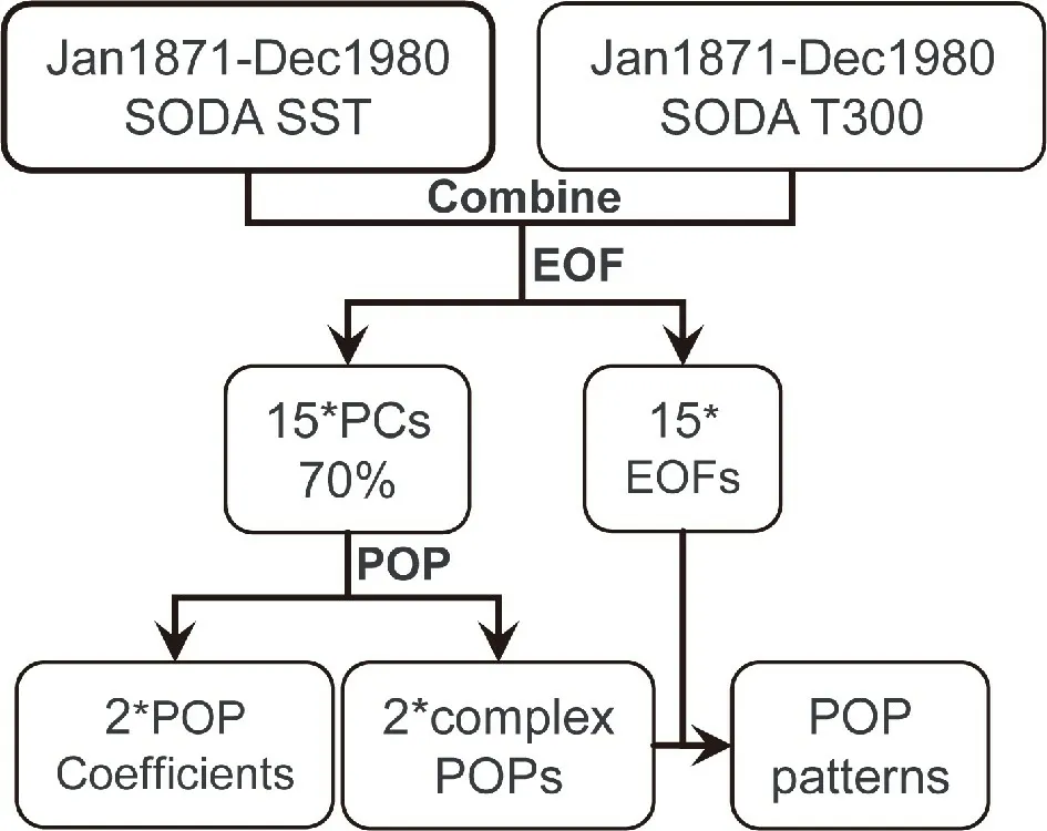
Fig. 1. Schematic diagram showing the POP-based analysis procedure to extract principal oscillation modes from the SODA dataset during 1871-1980.

The spatial patterns of SST and T300 for the real and imaginary parts for POP-2 are shown in Figs. 3a-d. Spatial patterns in Figs. 3a and d represent the peak phase, and those in Figs. 3b and c indicate the transition phase. Compared to the spatial patterns of POP-1 for the peak phase patterns, the SST and T300 anomaly centers of POP-2 are more concentrated in the central and northeast Pacific. This spatial pattern of SST is like the North Pacific meridional mode(NPMM), which exhibits significant periodicities of more than 5 years (You and Furtado, 2018). Moreover, the POP-2 temporal coefficients, Zr,2(t) and Zi,2(t), are shown in Fig. 3e together with ONI. The real part coefficient Zr,2(t) is strongly correlated with ONI. The imaginary coefficient Zi,2(t) leads Zr,2(t) by a quarter of the POP-2 period, i.e.,about 24 months.

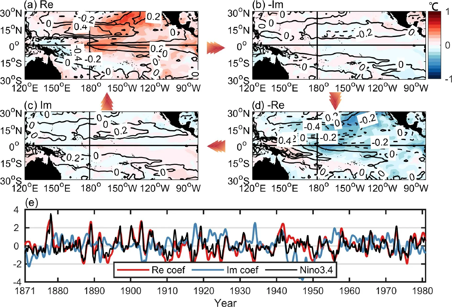
Fig. 3. The same as in Fig. 2, but for the second ENSO-related POP mode (POP mode-2; oscillation period: T = 8.1 yr).

In short, the POP-1 and POP-2 modes are two interannual-to-quasi-decadal modes related to ENSO. The real parts of temporal coefficients are highly correlated with the ONI, but the spatial patterns differ substantially. The POP-1 is the traditional ENSO-like mode, but the POP-2 is more like the NPMM pattern. These decomposed results are similar to those obtained using other Hadley Centre Sea Ice and Sea Surface Temperature data set (HadISST) and Ocean Reanalysis System 5 (ORAS5) dataset from ECMWF (not shown). As seen in their space-time evolution, both modes are critically important for ENSO evolution and prediction,which therefore are used for our POP-based prediction model formulation in the next section.

2.2.2. The POP prediction scheme

For a particular POP ( Pk=Pr,k+iPi,k), its condition at certain time t0is determined by the temporal coefficient Zk(t0)[Zk(t0)=Zr,k(t0)+iZi,k(t0)] . Then, the state at future time t0+τ can be calculated from

Here, λkis the corresponding eigenvalue of the POP. Thus,the prediction problem becomes one of estimating the POP coefficient Zk(t0) instead.

As described in section 2.2.1, the SODA analysis fields of interest were decomposed into individual modes during 1871-1980 using EOF and POP analyses, including the first 15 EOFs, PCs, and two ENSO-related POP modes. Next,we formulated the POP prediction model based on these results and evaluated the prediction performance using GODAS dataset. Specifically, SST and T300 anomaly fields at time t0from the GODAS dataset were projected onto the first 15 EOFs calculated from the SODA dataset to obtain the corresponding PCs. Then, the dot product between the vector PCs and the adjoint eigenvector D [ Dk=(P-k1)⊺] calculated from the SODA dataset was performed to obtain the POP coefficient Zk(t0). Accordingly, we calculated the POP coefficient Zk(t0+τ) at any lead time τ using Eq. (4).Finally, by combining the coefficient Zk(t0+τ) with POP spatial patterns, we obtained the predicted SST fields at time t0+τ, including the Niño-3.4 index. Further, we could evaluate the prediction skills from the POP-based model.

2.3. A CNN-LSTM model

ENSO prediction is a multivariate problem, which requires us to consider spatiotemporal information. Therefore, we formulated an ANN model, named as CNN-LSTM,by combining CNN with long short-term memory (LSTM)arithmetic (Hochreiter and Schmidhuber, 1997), which was used both as an independent model to predict ENSO and as part of the subsequent construction of the hybrid model in the next section. As is well known, CNN can detect the essential features automatically without any human supervision.The LSTM is well-suited to process sequential information,as it has a versatile potential for managing critical information with long periods and time delays. Several studies have demonstrated the effectiveness of LSTM in capturing the El Niño index non-stationarity (Guo et al., 2020; Wang et al.,2021). Following this reasoning, as shown in Fig. 4, we formulated a space-information extraction module (SEM) and a sequence analysis module (SAM) based on CNN and LSTM algorithms, respectively.

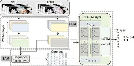
Fig. 4. Architecture of the CNN-LSTM model configured for the Niño-3.4 index prediction. The CNN-LSTM model consists of one input layer (the predictor as indicated by SST and T300), one space information extraction module (SEM)based on convolutional neural network (CNN) technique, one sequence analysis module (SAM) based on long short-term memory (LSTM) technique, and finally one output layer (the predictand). The input variables include SST and T300 anomaly fields between 0°-5°W and 50°S-50°N, from t0-11 months to the time t0 , in which t0 is the start month for the predictions. The ONI for the targeted prediction month is used as a variable for the output layer.

The training process of the model was divided into pretraining and fine-training processes, where CMIP6 data were used in pre-training and SODA data were used in finetraining process. The model processing procedures are identical for different inputs. Detailed processes are described as follows. The CNN-LSTM model used SST and T300 anomaly fields over (0°-5°W, 50°S-50°N) for twelve consecutive months as predictors, and the Niño-3.4 index was the targeted predictand as an output. Firstly, all predictors were interpolated to a 5° × 5° grid and then, as an input,fed to the SEM, which contained two parallel paths that extracted the important spatial features from SST and T300 fields, respectively. Each path of SEM had two convolutional layers whose convolutional filter number was 12 and size of 5 × 3. The outputs of the SEM were reshaped and spliced into a feature map, which was then incorporated as input to the SAM consisting of two LSTM layers meant to capture the overall information of the sequence. The second LSTM layer of the SAM was linked to a fully connected layer that contained 64 neurons and links to the final output layer. In addition, we trained the CNN-LSTM model with four different initialization parameters while keeping the model framework fixed. Finally, the predicted Niño-3.4 indexes from the four calculations were averaged to obtain the final values.

2.4. The hybrid model: POP-Net

So far, we have reviewed the POP analysis method,which can adequately extract propagating or standing patterns with specific periods from a complex system. Also, we constructed an ANN model, CNN-LSTM, for Niño-3.4 index prediction. We explored the combination of the two techniques to see whether a more effective ENSO prediction framework could be configurated. Consequently, we developed a hybrid model, named as POP-Net, which was composed of a CNN-LSTM module and a time-information extraction module (TEM; see Fig. 5). To facilitate the comparison, we set the CNN-LSTM module in POP-Net to have the same structure as the CNN-LSTM model presented in section 2.3, containing the SEM and the SAM as well. In addition, the TEM contained three-POP modes calculated using SODA SST and T300 data between (30°S-30°N,120°E-80°W) with 5° × 5° resolution during 1871-1980.The periods of these POPs are 1.8 yr, 4.0 yr, and 7.2 yr,respectively. Therefore, the TEM could extract the POP temporal coefficients at specific frequency bands from the anomaly fields. In these cases, the attributes of the POP-Net were derived from topological properties of the climate neural networks and knowledge of physical processes.

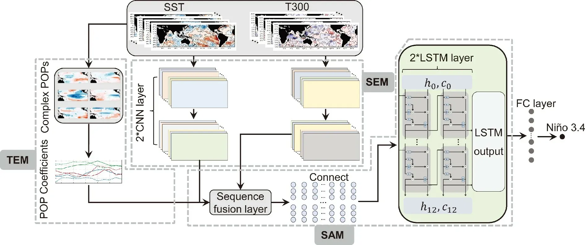
Fig. 5. The same as in Fig. 4 but for architecture of the hybrid model developed for the Niño-3.4 index prediction (POP-Net).The POP-Net model is composed of the POP analysis part and the CNN-LSTM model, with the former being added in by a time information extraction module (TEM). More specifically, the TEM is used to extract POP temporal coefficients at different frequencies from input SST and T300 data. Meanwhile, the convolution kernels in the SEM extract the spatial information from the input data (SST and T300). Then, the output data through the TEM and SEM processing are combined together as an input into the SAM to get more predictable information.

In the actual operations, when SST and T300 data from CMIP6 dataset in pre-training or SODA dataset in fine-training for twelve consecutive months were used as an input,the SEM could extract spatial information from the SST and T300 fields; on the other hand, the TEM calculates periodic POP temporal coefficients from input fields. Next, by combining the SEM and TEM outputs into the SAM, we obtained the final Niño-3.4 index predictive results. Just as the training process of the CNN-LSTM model described in the last section, we also trained the POP-Net with four different initialization parameters while keeping the model framework fixed. The final prediction values were obtained by averaging the results from the four calculations. This ensemble prediction method leads to a slight systematic improvement in prediction skills by canceling out the uncertainty within the individual calculation.

We used the AdaGrad optimizer (Duchi et al., 2011) to train the CNN-LSTM and the POP-Net models during 25 epochs, fix the learning rate to 5 × 10-3for the pre-training process, and set the training epochs to 20 and the learning rate fixed to 5 × 10-5for the transfer learning process. The CNN-LSTM and the POP-Net models were formulated separately for each targeted prediction month and lead time during the training process. As will be seen below, the POPbased analyses could be incorporated into an ANN-based model, transferring physical understanding and representation of ENSO processes into an improved prediction capability.

3. Assessments of ENSO predictions

During the model validation process, we used the Pearson correlation coefficient (PCC), the root mean square error (RMSE), and the mean absolute error (MAE) between the predicted and observed ONI values to evaluate the prediction performance of the models. The PCC measures the linear correlation, and the RMSE and MAE measure the differences or errors between the predicted and observed ONI.The PCC, RMSE, and MAE are calculated as follows:

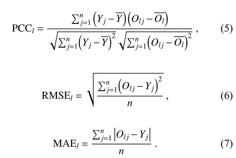
Here, n is the number of months during the validation period (1994-2020; taken as n=324); Yjand Oljdenote the observed and predicted ONI in the jth month at lead time of l month;andare their averaged values.

3.1. Hindcast results from POP and CNN-LSTM models

This paper focuses on the feasibility and effectiveness of the combined POP analyses and ANNs for ENSO prediction. In so doing, we first evaluate the prediction performance for the individual POP and CNN-LSTM models based on the GODAS dataset during 1994-2020; the validation results are shown in Fig. 6.

We calculated all-season PCC, RMSE, and MAE between the predicted and observed ONI values to assess the overall prediction performance. As shown in Fig. 6a, the POP model was able to make a valid prediction for only 6 months in advance (i.e., PCC＞0.5). In contrast, the CNNLSTM model is systematically superior to the POP model.The PCC skill of the ONI in the CNN-LSTM model is above 0.5 for a lead time of up to 15 months. Also, both RMSE and MAE are less than those in the POP model for all lead months. These results clearly indicate that the prediction error in the CNN-LSTM model is significantly smaller than that in the POP model. It is not surprising that such outcomes can be achieved, in practice, by using the complex ANNs such as the CNN-LSTM model, which can fit any nonlinear mapping given enough data theoretically (Scarselli and Tsoi, 1998). Many previous studies have also confirmed the advantages in using ANN models to make ENSO prediction over traditional linear statistical models (Tang and Hsieh, 2002; Wu et al., 2006; Guo et al., 2020).

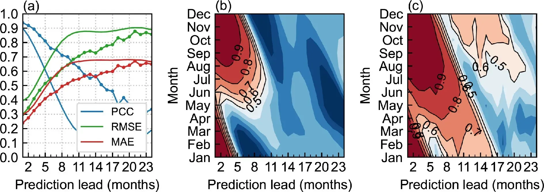
Fig. 6. ENSO prediction performance assessed for the POP and CNN-LSTM models. (a) The all-season Pearson correlation coefficient (PCC; blue), root mean square error (RMSE; green), and mean absolute error (MAE; red) are used to quantify skill of the ONI as a function of the prediction lead month; the POP model is denoted by unmarked solid lines and CNNLSTM model by solid lines with circular marks. The prediction skill of the ONI is also assessed by calculating the correlation coefficients as a calendar month in (b) the POP model and (c) the CNN-LSTM model. The contours highlight the correlation coefficients exceeding 0.5 in (b) and (c).

Figure 6b shows the correlation between the POPbased predictions and observed ONI as a function of start months and lead times. The distribution indicates an obvious SPB phenomenon, with rapid decreases in correlation coefficients when the prediction is initialized from boreal spring, increasing notably to later months at longer lead times. For example, the predictions initialized from May were only able to achieve a successful prediction for the following three months. In contrast, the CNN-LSTM model shows higher prediction skills for almost all calendar months than the POP model (Figs. 6b, c). Furthermore, skillful Niño-3.4 index prediction could be made for lead times of one year when initiated prior to boreal spring. So, the CNN-LSTM model substantially alleviates the SPB problem, which increases effective prediction time to 14 months when the prediction is started from May. Nevertheless,there still exists a “gap” in the correlation distribution when the CNN-LSTM prediction is initiated in boreal spring with the lead times of 5-7 months.

In short, the POP model, as a simple linear statistical model, has limited prediction ability. The CNN-LSTM model benefits from its powerful nonlinear fitting ability,showing significantly better prediction performance than the POP model. Even without excessive training manipulations, the CNN-LSTM model produces skillful ENSO predictions for lead times of up to 15 months, which is already better than most linear statistical or dynamical models (Barnston et al., 2012; Tippett et al., 2012; Tang et al., 2018;Ham et al., 2019; Zhang et al., 2021).

3.2. Hindcast results from POP-Net model

In section 2.4, we combined the POP analyses with the CNN-LSTM arithmetic to formulate a hybrid model, POPNet. The POP-Net model imposes additional constraint on the prediction process by incorporating the knowledge of characteristic ENSO space-time evolution patterns obtained from the TEM into the prediction. This combinational scheme not only reduces complexity of ANNs to extract helpful information from the input automatically, but practically improves the ENSO prediction performance. In this subsection, therefore, we will demonstrate the ENSO prediction performance using the POP-Net model.

The predicted Niño-3.4 index for 1-6 month lead times using the POP-Net model is shown in Fig. 7, together with the corresponding observed Niño-3.4 index. Here, only the predictions initiated from January of each year during 1994-2020 are shown. The results demonstrate that the POP-Net model can adequately predict the amplitude and variation of the Niño-3.4 index with at least 6-month lead times in advance.

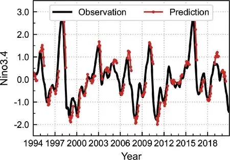
Fig. 7. Examples for the 6-month Niño-3.4 predictions in the POP-Net model (red) which are initialized from January of each year from 1994 to 2020; the observed Niño-3.4 index(black) is shown for comparison.

In addition, as expected, the hybrid model, POP-Net, further exhibits its ability to improve ENSO prediction skills,with correlation coefficients exceeding 0.5 up to a lead time of 17 months (Fig. 8a). Moreover, the POP-Net model further alleviates the SPB. As shown in Fig. 8b, the POP-Net model can make a valid prediction at least up to a lead time of 1 year when the predictions start from boreal spring,which is another significant improvement in prediction skill compared to the POP model and the CNN-LSTM model individually.

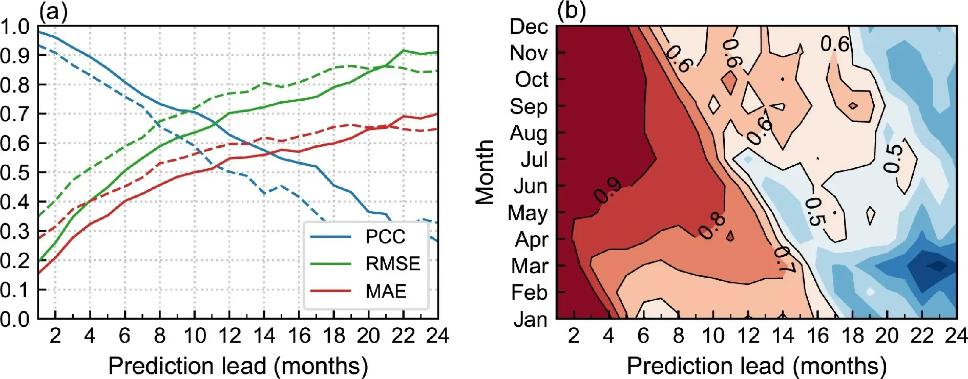
Fig. 8. ENSO prediction skill in the POP-Net model. (a) The PCC (blue), RMSE (green), and MAE (red) between predicted and observed ONI as a function of different lead times; two experimental results are presented: solid lines indicate that the input variables in the POP-Net model include both SST and T300 fields, and the dotted lines indicate the input variable includes SST only. (b) The correlation coefficients between the POP-Net predicted and observed ONI as a function of lead months and start months. Contours highlight the correlation coefficients exceeding 0.5 in (b).

To compare the prediction performance with different models more clearly, Table 3 quantifies the prediction skills in terms of the PCC, RMSE, and MAE at lead times of 3, 6,9, and 12 months, respectively. Evidently, the prediction skills of the POP-Net model are systematically superior to the other two models at different lead times. In addition, we conducted a sensitivity experiment to illustrate the effect of the input variables (SST and T300) on the model prediction skills. As shown by dashed lines in Fig. 8a, when the input variables are changed to include SST only, the ENSO prediction skill in the POP-Net model is significantly reduced. For example, the prediction has correlation coefficients exceeding 0.5 only up to a lead time of 12 months. Also, the prediction errors are larger than the experiment in which input fields include both SST and T300, indicating the vital role played by heat content in the long-term prediction of ENSO.

These results show that the inclusion of POP-based physical knowledge in the data-driven CNN-LSTM model does help improve the performance of ANN models. For example, the hybrid model can extend the effective lead time to 17 months, and further reduce the prediction errors,including significantly improved spring-time prediction skills (i.e., the alleviation of SPB). The combination of the POP analyses with ANN models is thus an effective method for predicting ENSO.

4. Case analyses and real-time prediction

The above results focus on overall assessments of the prediction performance among the three models. To see detailed prediction performances of individual ENSO events in these models, we present case analyses and realtime prediction during 2021-22 in this section.

4.1. Case analyses

Here, we select two typical ENSO events during the validation period: 2010-12 La Niña and 2015-16 El Niño events. These two events exhibit specificity and representativeness. For example, as shown in Fig. 9 for the observed ONI, a remarkable feature of the 2010-12 La Niña event is the “double dip” evolution of the Niño-3.4 SST in the fall of 2011 (Gao and Zhang, 2017). During 2010-12, the Niño-3.4 SST experienced a prolonged cold condition, with a La Niña event that occurred in the fall of 2010 and then a second cooling that occurred again in the fall of 2011. The 2015-16 El Niño event, which is one of the strongest El Niño events on record (Varotsos et al., 2016), displays some uniquely different evolution characteristics in 2014. In terms of prediction, most dynamic and statistical models have failed to predict the Niño-3.4 SST at long lead times(Zhang and Gao, 2016; Tang et al., 2018).

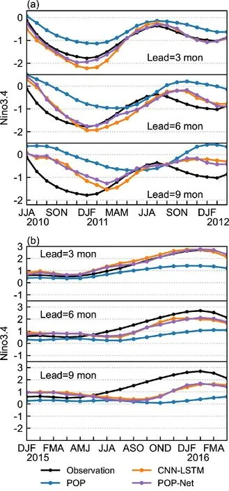
Fig. 9. Examples of predictions made for (a) the 2010-12 La Niña event (upper panel; the second-year cooling event) and(b) the 2015-16 super El Niño event (lower panel): ONI predicted at 3-, 6-, and 9-month lead times by POP (blue),CNN-LSTM (orange), and POP-Net (purple) models,respectively. The observed ONI is also shown in black.

Here, we further compare the prediction skills using the three models in these two cases; the predicted 2011-12 La Niña event at lead times of 3, 6, and 9 months is shown in Fig. 9a from the POP, CNN-LSTM, and POP-Net models.The results illustrate that the predicted amplitudes from each model gradually decrease as the lead times increase.The CNN-LSTM and POP-Net models have better prediction performance than the POP model at different lead times, demonstrating the advantage of nonlinear ANNs over linear statistical models. In addition, the predicted amplitude of the POP-Net model follows the corresponding observed Niño-3.4 index closer than the other two models,which indicates the effectiveness of combining POP analyses with ANNs in improving prediction skills. However,all three models fail to predict the second-year cooling at lead times of 9 months and more with a transitional point in the fall of 2011, which may reflect the deficiency of the ability to parameterize the critically important physical processes in the statistical models.

For the 2015-16 El Niño case, all three models can predict the variation in Niño-3.4 at least 9 months in advance(Fig. 9b). The CNN-LSTM and POP-Net models predict the amplitude closer to the observed values than the POP model. Nevertheless, the predictions made by the POP-Net model are in better agreement with the observation than the CNN-LSTM model at a lead time of 3 months; the differences in their predictions are small for longer lead times.

These two-case studies indicate that the ANNs have significant advantages over the linear statistical model for ENSO prediction. For the selected ENSO events, the ANN or hybrid models are demonstrated to have ability to improve prediction performance compared with dynamical or linear statistical models. However, the data-driven ANN model and hybrid model also face a challenge for providing accurate long-lead-time prediction for some specific ENSO events, such as the second-year cooling for the 2011-12 La Niña event at lead time of more than 9 months. The physics-based model can predict this event successfully by adjusting physical parameters (Gao and Zhang, 2017).

4.2. Real-time prediction

Finally, we perform a real-time prediction for SST condition during 2021-22. We use, as input data, monthly SST and T300 anomaly fields from the GODAS reanalysis during June 2020-May 2021. Then, we predict the Niño-3.4 index for the following 12 months by using data up to May 2021 to initialize the POP, CNN-LSTM, and POP-Net models. The predicted ONI is shown in Fig. 10. The POP model prediction results show that the Niño-3.4 SST increased but remained negative the next year. The CNN-LSTM and POP-Net model prediction results are similar; both show a trend of SST increase until August-September-October 2021 and then a decrease. The prediction from the two models indicates a maximum of the Niño-3.4 SST in the fall of 2021, and a minimum in the winter of 2021 or the spring of 2022, respectively. In general, the real-time predictions from all three models indicate that SST will be likely in neutral conditions in the coming year of 2022 in the tropical Pacific.

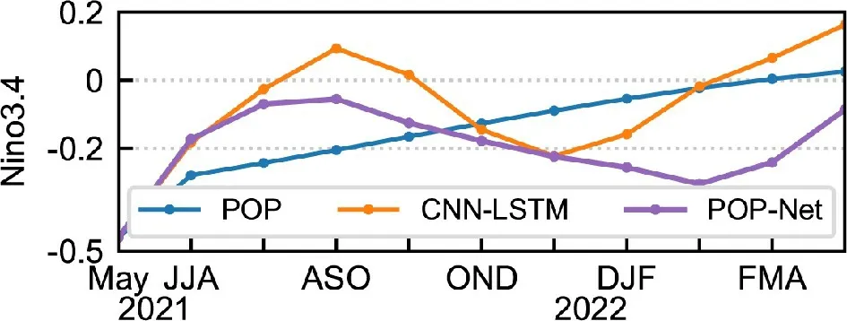
Fig. 10. Examples for one-year real-time prediction of ONI made by the POP (blue), CNN-LSTM (orange), and POP-Net(purple) models, which is initialized with data up from June 2020 up to May 2021.

5. Conclusions and discussions

ENSO represents a naturally reoccurring inter-annual climate fluctuation, which affects the climate system worldwide. ENSO prediction has been realized for several decades. However, large biases and uncertainties still exist in making predictions using the traditional approaches, including statistical and dynamical equation-based methods.Recent advances in deep learning method provide us with an opportunity to explore a data-driven approach to determine SST field in the equatorial Pacific. In this study, we have developed a hybrid prediction model by combining a deep learning framework (CNN-LSTM) with POP-based analysis method. Specifically, based on the periodicity, oscillation property and spatiotemporal correlation of ENSOrelated anomaly fields, POP analyses were first used to extract quasi-periodically propagating or standing patterns from the complex climate system. Then, we combined the CNN-LSTM with POP-derived data to formulate a novel hybrid model, named as POP-Net.

More specifically, the POP analysis was added in the CNN-LSTM framework by TEM, which was used to identify the periodically-varying POP patterns and corresponding temporal coefficients from SST and T300 anomaly fields. The TEM filtered out unrelated noise from raw data whereas useful signals of interest for ENSO prediction were retained. Synchronously, the convolutional layers of SEM in the CNN-LSTM extracted spatial information from SST and T300 fields to form feature maps. Then, by combining the TEM and SEM outputs into the SAM in the CNNLSTM, we obtained the final Niño-3.4 index prediction as an output.

We further compared the prediction performances using three models: POP model, CNN-LSTM model, and POP-Net, respectively. The correlation coefficients between predicted and observed Niño-3.4 index were calculated to quantify the skills. If a correlation coefficient value of 0.5 is considered as predictable measure for ENSO, the effective lead times for ENSO prediction were 6 months for POP model, 15 months for CNN-LSTM model, and 17 months for POP-Net, respectively. The prediction errors at each lead time (in terms of both RMSE and MAE) in POP-Net are less than those in POP and CNN-LSTM models.Moreover, the POP-Net also alleviated the spring predictability barrier. These improved performances are strikingly encouraging considering the fact that these prediction skills were assessed during the validation period including the 1990s, which exhibited low predictability in the tropical Pacific (Zhang et al., 2021).

The superiority of the POP-Net over the other two models in terms of ENSO hindcasts can be attributed to the usage of the POP-based analysis procedure to successfully enhance ENSO-related signals from input SST and T300 fields, which additionally acts to filter unrelated noises. In other words, this pre-processing acts as an "expert system"in computer science that reduces the difficulty for ANNs to search for predictable information in an automatic way.These practical achievements show the feasibility of using the enhanced periodic physical signals (prescribed from the POP analyses) to construct a robust deep learning-based model for the improved ENSO predictions.

In this study, we combined POP with artificial neural network to develop a new hybrid model for ENSO predictions.This paper describes the technical details of this new model and compares its prediction skill with that from conventional POP and artificial neural network models. The results indicate that this new hybrid model achieved an enhanced prediction capability without using an overly complex and advanced ANN algorithm, nor did it use too many training manipulations. In particular, the new model has the potential to improve the predictions of multi-year La Niña(i.e., 2010-12) and El Niño (2015-16), which are a great challenge to ENSO predictions (Gao and Zhang, 2017).However, there are notable issues that need to be addressed in the future. Although POP-Net shows clear advantages in predictions for case analyses and the spring predictability barrier compared to CNN-LSTM model, the overall prediction improvements were still quite limited with effective lead times of ENSO prediction being increased from 15 months to 17 months only. This is partly due to the greater difficulty in making lead-time prediction of more than one year in advance. Also, it may be related to the fact that we used a rather simple neural network construction in our preliminary applications, i.e., only two layers were used in the CNN and LSTM applications without taking other advanced construction techniques. Future studies are clearly needed to further improve ENSO prediction performance based on the POP-combined hybrid model by applying more advanced ANNs and effective information-encoding algorithms.

Another obvious weakness of the present study is the lack of mechanism analyses for the results. This is basically an interpretability issue, which is also a common challenge faced by current ANN modeling studies. In terms of ENSO predictions focused here, some specific questions need to be considered. For example, what are the differences in the aspects of ENSO feature extraction among POP, CNN and EOF that can lead to large differences in ENSO predictions as represented in the case studies and the SPB alleviation?How can our understanding of the ENSO mechanisms be used to improve the artificial neural networks for real-time predictions? In this paper, we have demonstrated that the prediction improvements can indeed be achieved by including the process-oriented analyses through the POP method.However, we still could not give a mechanism interpretation for the effect of POP-based information extraction on prediction performances from the neural network point of view. One possible action would be to use dynamical models, such as an intermediate coupled model (Zhang and Gao,2016), to further explore the mechanisms for which different POP modes affect ENSO predictions. Incorporations of data-based ANN and physics-based dynamical models are the next step to go forward in such ENSO-focused prediction challenges.

Acknowledgements.The authors wish to thank the two anonymous reviewers for their comments that helped to improve the original manuscript. The authors thank Dr. Yuchao ZHU for his help in providing us with CMIP6 products. This research is supported by the Strategic Priority Research Program of the Chinese Academy of Sciences (Grant No. XDA19060102), and the National Natural Science Foundation of China [NSFC; Grant Nos.41690122(41690120), and 42030410].