Stochastic optimal control for norovirus transmission dynamics by contaminated food and water
Anwarud Din and Yongjin Li(黎永锦)
Department of Mathematics,Sun Yat-sen University,Guangzhou 510275,China
Norovirus is one of the most common causes of viral gastroenteritis in the world, causing significant morbidity,deaths, and medical costs.In this work, we look at stochastic modelling methodologies for norovirus transmission by water, human to human transmission and food.To begin, the proposed stochastic model is shown to have a single global positive solution.Second, we demonstrate adequate criteria for the existence of a unique ergodic stationary distribution >1 by developing a Lyapunov function.Thirdly, we find sufficient criteria Rs <1 for disease extinction.Finally,two simulation examples are used to exemplify the analytical results.We employed optimal control theory and examined stochastic control problems to regulate the spread of the disease using some external measures.Additional graphical solutions have been produced to further verify the acquired analytical results.This research could give a solid theoretical foundation for understanding chronic communicable diseases around the world.Our approach also focuses on offering a way of generating Lyapunov functions that can be utilized to investigate the stationary distribution of epidemic models with nonlinear stochastic disturbances.
Keywords: stochastic norovirus model, stochastic transmission, stochastic perturbation, stochastic stability,stochastic optimal control
1.Introduction
Acute viral gastritis is still one of the most common illnesses on the globe.Human noroviruses (NoV) have gained growing attention in recent decades,despite the fact that they are caused by members of a number of viral families.The NoV is spread through the faecal oral route, which involves contact with human faeces; they could also be released in vomitus.Specific transmission of the NoV can occur directly between persons or indirectly via ingestion of infected water or food, or contact with fomites, based on these two decisive sources.[1]Although the proportional importance of each of these channels is debatable,it is widely acknowledged that the NoV group alone is responsible for a significant amount of the global foodborne disease burden.[2,3]
The most common meals linked to sporadic instances and outbreaks of viral gastroenteritis are three[4]
A1 During production, molluscan shellfish became infected.
A2 Contaminated fresh products during harvesting, manufacture or packing.
A3 During the processing of prepared or ready-to-eat(RTE)foods,contamination occurred.
Infected food workers’ poor personal hygiene habits are the source of contamination for prepared foods, which is the type of product most frequently associated in NoV outbreaks.Many factors influence the risk of contamination posed by infected food handlers,including the stage of clinical infection,which influences the degree of virus shedding,health and hygiene habits, virus removal and/or inactivation efficacy, virus perseverance,ease of virus transfer and a variety of individual characteristics.Contaminated hands, and to a lesser extent,contaminated surfaces,clearly play an important role as virus givers and recipients.[5]
Many elements can aggravate norovirus transmission and the resulting sickness.Over half of infections occur during the winter months, indicating that the virus has a high seasonality.[6]Seasonal variation is attributed to environmental factors as well as population behavior.Norovirus,for example,is more easily spread at cooler temperatures and may be boosted by greater rains.[7,8]Other factors in the population can influence the intensity of norovirus outbreak.The disease affects people of all ages,although it is more common in children under the age of five.[9]According to serological studies,the first norovirus infection occurs in childhood.Individuals who are elderly or immunocompromized are more prone to develop serious problems and could die.[9,10]As a result,while infection is self-limiting in healthy people,the consequences for certain groups with high-risk can be devastating.It has been shown that these groups can shed for far longer periods of time, potentially prolonging an outbreak.[11–14]
Mathematical modelling is an important tool for studying disease transmission and forecasting the efficiency of novel control methods.[15,16]Mathematical models can establish a compromise between biological reality in their depiction of infection’s natural history and the strength of their data link.Norovirus models built at various sizes, out from outbreak to population levels, have discovered a wide range of reproduction numbers estimates.Environmental noises are always the main factors in real-world systems and in biological phenomena.Variations in the environment have a significant impact on the spread of the NoV epidemic.[17]Because of the unpredictability of person-to-person connections or other aspects of population,an epidemic growth and its transmission is fundamentally unpredictable.As a result, the epidemic’s condition is influenced by the environment’s variety and randomness.The NoV infection is an excellent example of epidemic growth and dissemination being unpredictable due to unpredictability of contaminated water or food or person to person contact.
Parasite spread and persistence are influenced by environmental changes.The role of stochasticity has a large impact on epidemiology, fluctuations might be random but positively autocorrelated, such that the environment is comparable to the recent past(red noise),or random and uncorrelated with the past(white noise), the stochastic noises, can be analytically calculated by considering aerial image as a probability density function of photons.[18–22]The deterministic and the stochastic modeling techniques are the two main types of approach for epidemic modeling.When it comes to mathematical modelling of biological phenomena,stochastic differential equation models are preferable to deterministic models because they can provide a higher level of realism than their deterministic versions.[23–26]Because we may build up a distribution of the anticipated outcomes, such as the number of infected classes at timet, by running a stochastic model several times,it produces more valuable output than deterministic models.A deterministic model, on the other hand, will only provide a single outcome irrespective of the experiments thus far.For the description of the viral dynamics of NoV,many deterministic epidemiological schemes have been suggested,for instance see Refs.[27,28].The vast majority of NoV transmission models employ a compartmentalized approach,in which the population is divided into disease states.In this connection, the population is usually split into three groups: susceptible, infected, and recovered (SIR).An exposed or latent compartment (E) is frequently included in norovirus models.The exposed compartment is required to measure the efficacy of controls aimed at infected people.[29,30]As a result,only a few writers have investigated the dynamics of noise in NoV models.[31]Until now, to the best of the knowledge of the authors, none of the previous studies reported to prob NoV transmission due to contaminated water or food by employing mathematical modeling.
In this study, we suggested a stochastic epidemic model for understanding the transmission dynamics of the NoV virus(particularly the long-term behavior) in a shifting population context with contaminated water and food.We divide the entire community into five distinct groups.HereS(t) denotes the susceptible individuals, the variableI(t) stand for the infected/infectious individuals,R(t)represents the recovered individuals,W(t)represents the concentration of the NoV bacteria in the contaminated water and the last classF(t)represents the concentration of the NoV bacteria in the foods while considering the environmental fluctuations.Besides,the proposed NoV model take into consideration the following assumptions:
A2-1 The state variables and the parameter(s) used in the model are nonnegative.
A2-2 Per unit of time, the mean number of contacts is “c”.
A2-3 Every subject in the SIR compartment is exposed to the same risk of moving to another compartment and same forWandFcompartments; the probability distribution of moving between the classes are subject to the exponential distribution and the expected average time took in a class can be calculated by considering the inverse of that parameter in an exponential distribution.
A2-4 The model fits an epidemic out-break within a closed population if the whole population can be regarded stable and stationary with the population size remaining constant (without discharges,deaths or inflow into the population).
A2-5 If the demographic is open, additional transition coefficient d must be included in the model to account for new entries,discharges,and deaths.The maintenance of an endemic state within a population requires an open population.
A2-6 The total populationN(t)=N•is a constant andN•is independent of timet.
A2-7 We used a set of functionsWi(t)fori={1,...,5}to incorporate environmental noise into the model withWi(0)=0 as the standard Brownian motion and α1,α2,α3,α4,α5>0 representing respective intensities of the environmental noises.
Assuming assumptions A2-1–A2-7 and further considering that the stochastic perturbations are directly related toS(t),I(t),R(t),W(t), andF(t).Based on the above assumptions,we obtained the following stochastic model:


where the description of parameters is presented in Table 1.Furthermore,the time-dependent functionsWi(t)fori=1,2,...,5 represents independently the Brownian motions andstand for the intensities of these noises with αi>0 for all values ofi.
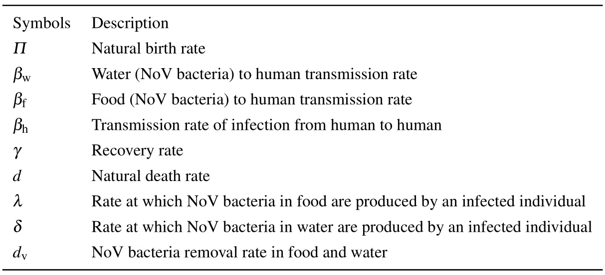
Table 1.Parameters description.
Now,on the basis of model(1)we may proposed the following questions:
Q1 Is white noise affect the dynamics of a disease caused by NoV?
Q2 What role contaminated water plays in the spreading of disease due to NoV?
Q3 What role does contaminated food play in the transmission dynamics of NoV?
Q4 What are the criterion that ensure the existence of stationary distribution?
Q5 What conditions are required in the stochastic optimal control?
The organization of this paper are arranged as follows.In Section 2, we provide the existence/uniqueness of the unique positive global solution after stating a few lemmas.By using a single condition, we proved the persistence of the disease in Section 3.Section 4 of this study focuses on establishing sufficient criteria ensuring the existence and uniqueness of the ergodic stationary distribution.The stochastic optimal control problem is presented and investigated rigorously in Section 5.The theoretical findings are verified numerically and the results are displayed in Section 6.The study was concluded in Section 7 by stating the conclusion and future research directions.
2.Global positive solution
The system (1) describes the dynamics of a biological population.Hence, the population sizes should be nonnegative and bounded.For this reasons,we first establish the global existence,positivity,and boundedness of solutions for the proposed model.
Theorem 1The solution of the system (1), that is,(S(t),I(t),R(t),W(t), andF(t)) is unique fort≥0 and for an initial value (S(0),I(0),R(0),W(0),F(0)) ∈, It will continue to exist inR5+with unit probability, namely(S(t),I(t),R(t),W(t),F(t))∈R5+,∀t≥0.
ProofClearly the coefficients are continuous locally Lipschitz for (S(0),I(0),R(0),W(0), andF(0)) in, which show that the solution (S(t),I(t),R(t),W(t),F(t)) is unique and local in the interval[0,τe)for anyt,here τestands for the explosion time(see for more detail in Refs.[32,33]).Proving τe=∞guarantees that the solution is in fact global.Letk0be a constant and assume that it is non-negative, and be a large number, so that (S(t),I(t),R(t),W(t),F(t)) lies in [k0,1/k0].Then by definingk≥k0and

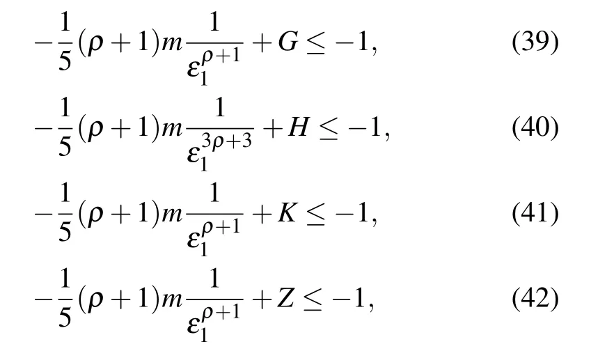
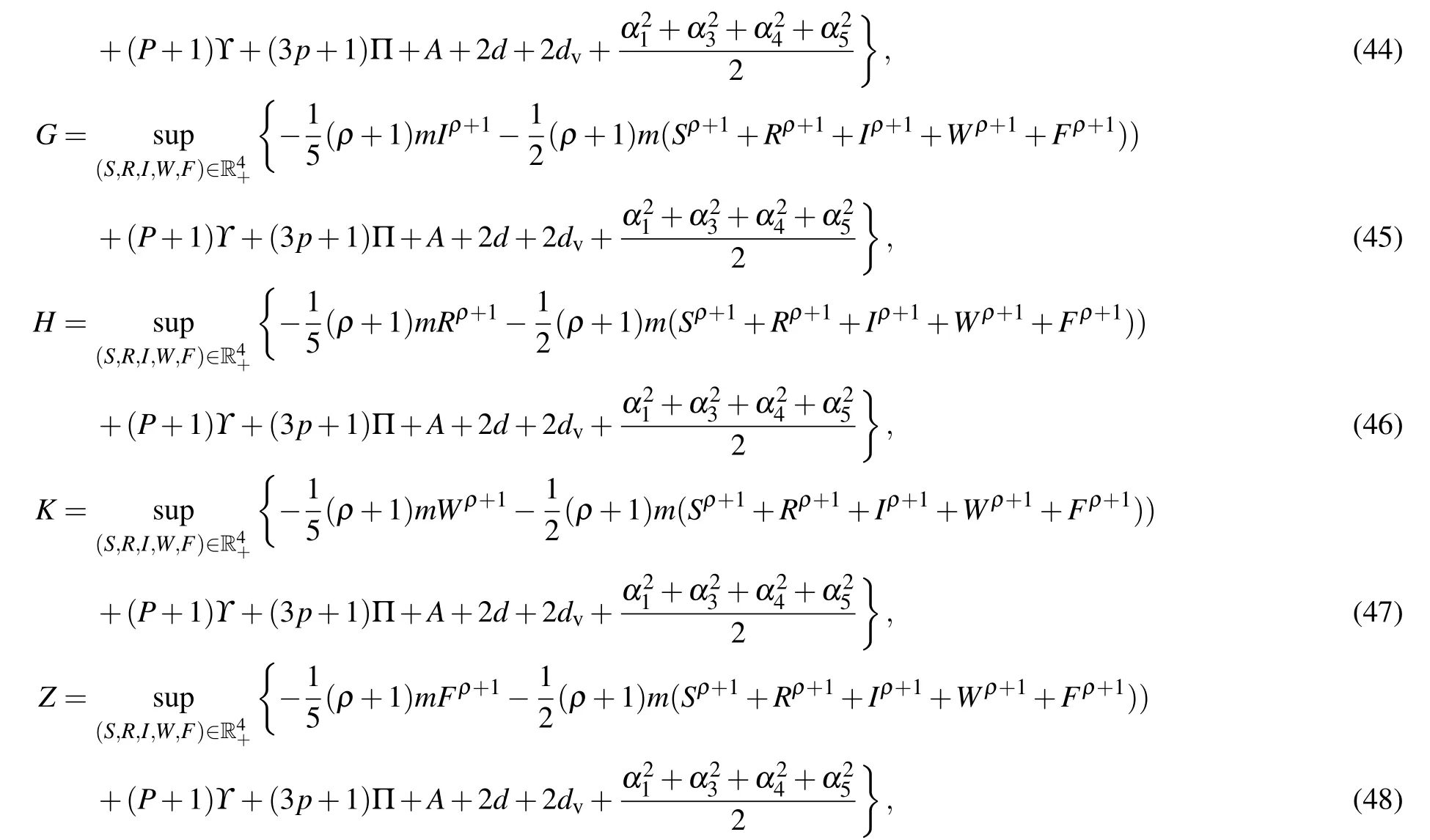
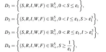
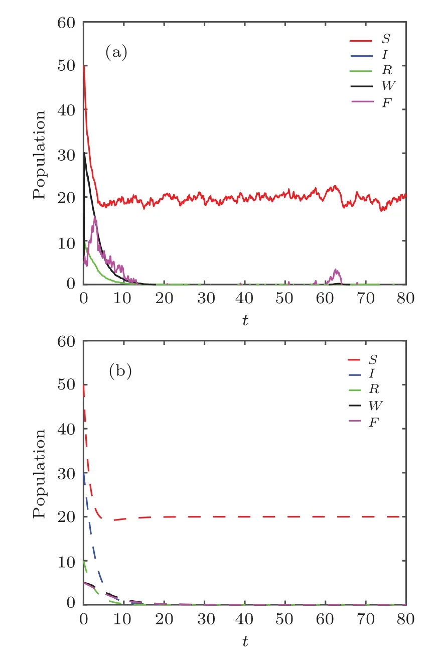
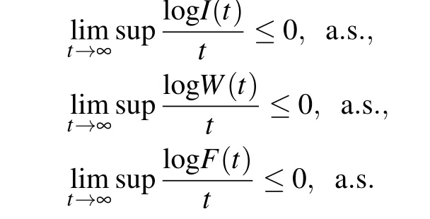
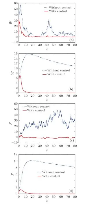
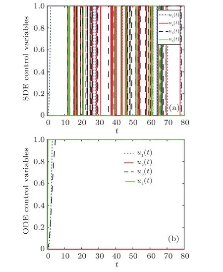
We now set infφ =∞, as φ is the empty set.Here τkis increasing askapproaches to ∞.Assume that τ∞is the limiting value, that is,limk→∞with τ∞≤τea.s.Here it is enough to show that τ∞= ∞a.s., then τe= ∞, which proves that(S(t),I(t),R(t),W(t),F(t))∈a.s.,for everyt≥0.We verify that τe=∞a.s.If this not holds, then there will be a pair of constants 0 So an integerk0≤k1will be there,such that we have the following expression: P{T≥τk}≥ε, for allk1≤k. Define the following Lyapunov function: whereCwill be determined later. Applying Itˆo formula to Eq.(4).We assume thatk≥k0and choosing arbitraryT>0,then In Eq.(5),we define theG:by the assertion Let β = Max{βw,βf}, then chooseC=dv/β, such thatCβ −dv=0, from Eq.(2), we know thatS(t)+I(t)+R(t)+W(t)+F(t)≤1,then we have Accordingly Set Ωk={τk≤T},fork1≤kby Eq.(3),it could be noted thatP(Ωk)≥ε.Noticing that for every ω ∈Ωk,at least oneS(τk,ω),I(τk,ω),R(τk,ω),W(τk,ω),F(τk,ω),exists,which is equal tokor 1/k.SoS(τk,ω),I(τk,ω),R(τk,ω),W(τk,ω),F(τk,ω),is not less thank−logk−1 or 1/k+logk−1.Moreover Following Eqs.(3)and(8),we obtain where the function 1Ω(ω)is called the indicator function of Ω.Assumingk→∞goes to the contradiction,i.e.,TM,thus τ∞=∞a.s.and hence end the proof. One of the most important concerns in epidemiology is how to manage disease dynamics in order to eliminate it permanently.In this section,we will discuss sufficient conditions for the elimination of the disease in model(1).For the sake of clarity,we define Lemma 1Let (S(t),I(t),R(t),W(t),F(t)) be the solution of the model(1)with the initial value Then Furthermore,if and then For proving Lemma 1, one needs to follow the same approach used in the proof of Lemma 2.1 and Lemma 2.2 in the work of Zhao,[34]and thus we omit it. Next we are going to discuss the extinction and therefore first we define the basic reproductive parameter denoted as Rsfor stochastic model as stated by Eq.(1) and defined by the following expression: Theorem 2Let(S(t),I(t),R(t),W(t),F(t))be the solution of system(1)with(S,I,R,W,F)(0)∈R5+,if Rs<1,then any solution of the stochastic hepatitis B model(1)obeys namely the disease extinct with probability one. ProofBy directly integrating the proposed system (1),the following system of equations can be obtained: From the second last Eq.(14),we can easily obtain Let and in the similar way from the last Eq.(14),where we can obtain Applying Itˆo formula on the second equation of system(1),then we can get The following equation can be easily obtained if we integrate Eq.(17)over[0,t]and divide the resultant byt,i.e., Substituting Eqs.(23)and(24)into Eq.(18),then we can get Moreover wherei={1,2,3,4,5}which is a local continuous martingale andMi(0)=0.Applying the limitt→∞and using Lemma 1,we have And in a similar way we can say limt→∞supMw(t)=0 and limt→∞supMf(t)=0. If Rs<1 is satisfied,then equation(19)becomes A direct result from Eq.(21)is given by By substituting Eq.(22)into Eqs.(23)and(24),and utilizing the properties of limt→∞supMw(t)=0 and limt→∞supMf(t)=0,then we can get Moreover,by considering the the first equation in model(14),integrating it between[0,t]and dividing byt,and finally using Eqs.(22)–(24),we obtain Thus implies that In a similar way,we can get which proves the complete result. In studying epidemiological dynamics,we are concerned not only with situation in which the disease extinct out of the population, but also dealing with the prevalence of the disease.For model (1), there is no disease present equilibrium of the model.Therefore, in this portion of the study, we use the theory of Khasminskii[35]to focus on the existence of a stationary distribution,reflecting whether the disease is prevalent.LetX(t) be a homogeneous “Markov” techniques in thed-dimensional real line space Rd, which satisfies the autonomous equation It is well known that the diffusion matrix corresponding to Eq.(28)has the form Lemma 2[26]LetU∈Rdbe a bounded open domain with continuous boundary Γ,which has the given characteristics: H1 There exists a positive constantM. for allx∈Uand ξ ∈Rd. H2 There is aC2-function 0 ≤VsatisfyingLV<0 for anyx∈Rd−U. Then the “Markov” techniquesX(t)have a unique ergodic stationary distribution π(·).In this situation, where the functionf(·) is considered to be integrable w.r.t measure π. Theorem 3Assume that then for a certain initial value(S(0),I(0),R(0),W(0),F(0))∈, model (1), has a unique stationary distribution π(·) and the ergodicity holds. ProofFrom Eq.(29), we know the diffusion matrix of system(1)has the form According to Lemma 2, we only need to verify the conditions H1 and H2.Let then we have for all(S,I,R,W,F)∈:=[1/n,n]5provided thatn∈Z+is sufficiently large.Note that ξ =(ξ1,ξ2,ξ3,ξ4,ξ5)∈R5.Hence,the condition H1 holds.To verify condition H2,we denote V(S,I,R,W,F):=PV1+V2−lnS−lnR−lnW−lnF, where V1:=S+R+I+W+F−C1lnS−C2lnIandV2:=(S+R+I+W+F)ρ+1. Pand ρ are positive constants satisfying the conditions andC1andC2are unknown constants to be determined at later stages. letC1(d+)=Π,andC2(γ+d+)=Π,then we can get Then we can obtain Similarly,we have Moreover,we get Therefore,we can easily check that where Construct the following compact subset where ε1is sufficiently small constants and in the R5+Dε1,they satisfy whereD,F,G,H,K,Zare real and positive and are defined as follows: and For sufficiently small ε1, condition (35) holds due to −Pb+B≤−2.For convenience of calculation, we divide the setinto eight domains, then we will illustrateLV≤−1 on the set R5+Dε1. Case 1If(S,R,I,W,F)∈D1,we obtain By using inequality(34),we obtainLV≤−1 for all(S,R,I,W,F)∈D1. By making use of inequalities (35)–(37), and being a similar way to the proof of Case 1, we make the conclusion thatLV≤−1 for all(S,R,I,W,F)∈D2,(S,R,I,W,F)∈D3,(S,R,I,W,F)∈D4,(S,R,I,W,F)∈D9,and(S,R,I,W,F)∈D10. Case 2If(S,R,I,W,F)∈D5,we have that According to inequality(38),we achieveLV≤−1 for all(S,R,I,W,F)∈D5.Furthermore, being similar to the proof of Case 2 and combining with Eqs.(39) and (40), the conclusionLV≤−1 can be obtained for all (S,R,I,W,F)∈D6,(S,R,I,W,F)∈D7,and(S,R,I,W,F)∈D8. On the basis of the above discussion,it follows that which proves the condition (H2) of Lemma 2, and model (1)has one and only one stationary distribution and thus the ergodicity holds. In recent years, optimal control strategies have received a lot of attention.These techniques are used to provide the best control solutions for a variety of diseases.The principle of control theory is a useful tool for determining the appropriate information circulation technique.[26,36]In the discipline of optimality,there is a large literature and numerous applications in the fields of dynamical systems,economics,and mathematical physics.[37]We recommend the readers to see Ref.[38]for a discussion of necessary optimality criterion and other related conclusions in state restricted control systems. The optimum disease-control approach is one that has the greatest chance of reducing the number of infected people at the lowest expense.The basic steps are summarized as follows: linking a model to a real-world problem.This stage is not an essay task due of an absence of physical understanding related to the phenomenon.In many circumstances,we just have experimental data and some literature results to work with.To identify a well-adapted model, extensive bibliographic research and several trials with various mathematical models are required.The mathematical framework will need to be modified to conform to the experimental data,therefore a first representation is rarely convenient.Liu and Meng also looked at the best harvesting techniques as well as the dynamical elements of the stochastic delay model.[39,40]The authors derived optimal harvesting techniques and the upper limit of expectation of sustainable yield using optimal harvesting theory, the method of Hessian matrix and ergodic theory,see Refs.[26,35]and cited work therein for recent updates on the stochastic optimum control strategy. As a result,we design stochastic optimal strategies based on the preceding literature by including the following timedependent control variables and some other features into model(1). A1 The control measureu1represents the isolation of water and food (NoV bacteria) and infected populations.The prominent role of the controlu1is to decrease water (NoV bacteria) transmission rate βwand transmission rate βfdue to food NoV bacteria. A2 The control variableu2physically shows the treatment of NoV infected people.With the help of this control measure,the infected population will tend to decline and will ultimately get recovery. A3 The control variableu3describes an effective process through which growth of water NoV bacteria could be controlled.This control aims to minimize the size of water NoV bacteria population. A4 The control variableu4is used to control food NoV bacteria population and via this control,one can reduce the rapid growth of food NoV bacteria. Based on the aforementioned assumptions, as well as the four control variablesu1,u2,u3, andu4, the associated stochastic controlled version(1)is of the form satisfying the conditions The following vectors are defined for the ease of use: Moreover,vector which accumulates the initial data is given by wherefandgare also vectors with components of the form whereg1=α1S,g2=α2I,g3=α3R,g4=α4W,g5=α5F. We consider a cost function that is quadratic in nature where the notionsAi,Bi,andkjfori=1,...,4 andj=1,...,5 denotes the positive real numbers. Our main objective in this work is to find the control vectoru∗(t)=in such a way that whereUis the set of admissible control(s)and is defined as whereli=fori=1,...,4 are real and positive which denotes the respective maximum values of the control functions.For utilizing the stochastic version of maximum principle,first of all,it is necessary to define the Hamiltonian functionHm(x,u,p,q)of the form where 〈·,·〉 stands for the Euclidian inner product while the vectorsp=[p1,p2,p3,p4,p5]′andq=[q1,q2,q3,q4,q5]′denote the adjoint vectors.The following results can be obtained easily from the standard maximum principle heres∗denotes an optimal curve ofx(t).The condition on the state variable att=0 andt=tfof Eqs.(65)and(66)are respectively.As, equation (67) indicates that the optimum value of the control(s)u∗are functions of the adjoint and states variables,thus,we can write here φ is an unknown function and can be found with the help of Eq.(67).Therefore, the corresponding Hamiltonian function will takes the form By considering the derivatives of the Hamiltonian w.r.t the state variables (i.e.,S,I,R,W, andF), we get system of ODEs describing the dynamics of the adjoint variables of the form supported by the additional conditions at initial and final time wherep1(tf)=−k1S,p2(tf)=−k2I,p4(tf)=−k3R,p4(tf)=−k4W,p4(tf)=−k4F.Now differentiating the Hamiltonian equation with respect tou1,u2,u3,andu4,we get the following characterization of the controls[26,36] We will slightly change the controls in a dynamic system to achieve the goals when dealing with the optimal control problems.We used ordinary differential equations for the representation of the system and chooses the structure and limits of the control measures in order to build up and solve the optimal control problem as shown by Eq.(60).By using the subsequent equation (61), we designed the objective functional for the problem.To create an objective functional that is relevant, it is required to balance competing factors in the functional and decide whether or not to add terms in the end.Because the optimal control results are greatly influenced by the objective functional being chosen, selecting one is a critical task that should be approached with caution.If there are more than two components involved in the objective functional, weights should be only assigned to those components based on their respective relevance.Before applying the maximum principle,[40]first of all, we must use the compactness theory for proving the existence of the optimal controls.This argument is based on the set of controls being utilized,which are commonly continuous piecewise or Lebesgue measurable and bounded functions.After that, one can design a maximizing/minimizing sequence of controls and relative state sequences, as well as prove convergence in the proper feasible space,to prove that the objective functional is bounded for all feasible controls.The challenge of finding a control that maximizes the objective functional subject to the state ordinary differential equation(ODE)and initial values is converted to the problem of optimizing the Hamiltonian point wise using this principle.According to Ref.[40],we may define the Hamiltonian as the following expression: Hamiltonian=(integrand of the objective functional)+(adjoint)(RHS of differential equations). For maximizing the value ofH, we must consider the derivative ofHw.r.tufor deriving the optimality conditions.To derive the adjoint system, we will take the partial derivative ofHw.r.t to the state variables and the system will be supported by the condition(s)which are called the transversality conditions as described by Eq.(73). In applied problem particularly problems in mathematical modelling, one must verify the model predictions or theoretical results through simulating the model.In this work,we intend to simulate model(1)with the help of quickly converging numerical schemes.The simulation to be presented here are mostly relevant to qualitative aspects of the study and the assumed parameters are justified biologically.The standard RK-4 method is used and the following scheme for the proposed model is presented: The terms ζi,j(i=1,...,5)are the independent random variables(Gaussian)havingN(0,1)distribution,whereas,the time step is Δt.Further,αifori=1,...,5 are positive real numbers and physically they describe the values of the white noises. To perform numerical simulation and biological feasibility of system(1),we must assume parameter values and noise intensities from Examples 1 and 2.The initial compartmental values of susceptible,infected,removed,water,and food NoV becteria are also shown in Examples 1 and 2.The desired time interval is[0,80]. Theorem 2 establishes sufficient conditions for the extinction of the disease and the theorem is proved using stochastic stability theory.Simulations suggest that only if Rs<1 then conclusion of Theorem 2 will hold and in such cases,the disease will tend to dies out with probability one.Solution curves of both the models will tend to disease-free fixed point and this assertion is supported by Fig.1 which shows that the disease will extinct within a finite time. Fig.1.Trajectories of stochastic system (1) with its corresponding deterministic version:(a)stochastic tobacco smoking model and(b)deterministic tobacco smoking model. On the other hand,Theorem 3 ensures the persistence of the disease whenever the dynamics of the disease was modeled by the proposed model.By using the values of parameters from Example 2 we calculated that R0s>1.As hypothesis of Theorem 3 is satisfied and the disease must persist in such a case.As shown in Fig.2, under dynamics of model(1)the disease will tend to persist and hence for the proposed model,there exists an ergodic stationary distribution. Fig.2.Trajectories of stochastic system(1)with its corresponding deterministic version: (a) S(t)–susceptible individuals, (b) I(t)–susceptible individuals, (c) R(t)–susceptible individuals, (d)W(t)–concentration of the NoV bacteria in water,(e)F(t)–concentration of the NoV bacteria in food. Fig.3.The probability distribution histograms of (S,I,R,W,F) for the stochastic model(1):(a)S(t)–susceptible individuals,(b)I(t)–infected individuals,(c)R(t)–recovered individuals,(d)W(t)–concentration of the NoV bacteria in water,(e)F(t)–concentration of the NoV bacteria in foods. We simulated the model for about 1000 times and obtained the mean extinction time for the infectious class.If we choose different values of the intensities, we will obtain different values of mean extinction time.We concluded that there exists an inverse relationship between the mean extinction time and noise intensities which is the key result of Theorem 3.The histograms shown in Fig.3 depict the probability distribution of each compartment. Example 1We choose the parameters as Π = 10,βw= 0.02, βf= 0.02, βh= 0.5, γ = 0.04,d= 0.5, λ =0.02, δ = 0.03,dv= 0.2 for the initial value, we choose(S(t),I(t),R(t),W(t),F(t))=(50,30,10,05,05)for noise intensity α1=0.150,α2=0.100,α3=0.115,α4=0.110,and α5=0.90.The basic reproduction number Rs<1 can be easily calculated and according to Theorem 2 the solution of model(1)must obey This suggests that in such a circumstance,the disease will be eradicated from the population, as seen in Fig.1, where numerical simulations back up our theoretical findings. Example 2In a similar way we choose the parameters as Π =2.5, βw=0.3, βf=0.3, βh=0.5, γ =0.06,d=0.1,λ =0.05,δ =0.06,dv=0.2 for the initial value,we choose(S(t),I(t),R(t),W(t),F(t))=(50,30,10,05,05)for noise intensity α1= 0.100, α2= 0.99, α3= 0.80, α4= 0.75, and α5=0.90 for stationary distribution of model (1).We calculatedand found that it exceeds unity.The statement of Theorem 3 is about the persistence of the disease and figure 2 is in the support of this statement.In the same way,we showed analytically that the model has an ergodic stationary distribution and numerically figure 3 confirms this assertion. Here,the notionS(t)stands for susceptibles,I(t)denotes the infected individuals,R(t)denotes the recovered individuals,W(t) represents the concentration of the NoV bacteria in the contaminated water, and the last classF(t)represents the concentration of the NoV bacteria in the foods. We will show some graphical results on the optimal control theory of system (1) in this subsection.The simulation will be carried out here again by using the fourth-order Runge–Kutta technique.We choose the parameters values as those in Example 2. Both with the control and without control, our problems were simulated and the results are shown in Figs.4(b), 4(d),and 4(f),which describe the dynamics of susceptible,infected class,and recovered individual by considering the corresponding deterministic version of system (1).The key aims of the control section is shown by the figures and the infected and susceptible populations will tend to decline and similarly,the recovered one will build up.Also, it is clear form the figures that the water and food NoV bacteria will tend to decrease(see Fig.4). Besides, the controlled and without control version of system(1)is simulated with the help of RK4 tools.The best technique is to solve approximately the states and adjoint system while keeping the transversality criteria in mind.The state system (70) is solved initially with the help of RK4 method and then an iterative procedure is presented for the state equations.The adjoint equations along with transversality conditions (71) are solved by backward method.We updated the control variables with the help of convex combination of the control obtained previously and the new controls (73).The iterative procedure was repeated until the two successive approximations are enough close to each other. The computed results for optimal control under strategies 1 and 2 are reflected in Figs.4(a), 4(c), 4(e), one can observe that the control strategy results a decrease in the number of susceptible and infected under model (1), and from Fig.5(a), we can see that the recovered ones are increasing, we can clearly see in Figs.4 and 5.Furthermore, figure 6(a) represents the dynamic of the optimal control variables of model (1).Clearly, the difference between the two cases is visible,see Fig.6. Fig.5.Simulations for the stochastic models(1)and its corresponding deterministic version,both with and without controls: (a)W(t)with and without control for stochastic system, (b)W(t) with and without control for deterministic system,(c)F(t)with and without control for stochastic system,(d)F(t)with and without control for deterministic system. Fig.6.Simulations of control variables for the stochastic models(1)and its corresponding deterministic version: (a)trajectories of optimal control variables for stochastic systems and(b)trajectories of optimal control variables for deterministic systems. In this work,we formulated a new stochastic model which describes the dynamics of NoV bacteria spreading through food and water.After studying basic properties of the model,we presented sufficient criterion for the permanence and extinction of the infection.By considering the possible variations in noises,we studied the behavior of the threshold parameter.We showed that the infection will tend to dies out of the population for Rs<1.Utilizing the techniques of stochastic Lyapunov,sufficient condition is derived for the ergodicity of the model and it is proved that infection will be permanent in the population if we keep>1.We considered a few external control characteristics of the infection and rigorous analysis for the stochastic control model was presented.By using the stochastic RK-4 method,we depicted sample curves for stochastic models both with and without controls.In parallel, we provided sample curves for the corresponding ODE model and compared the results with stochastic predictions.We find that the proposed control strategies can prevent and control the disease in a cost effective way.Using this approach, we conclude that the norovirus transmission dynamics by contaminated food and water reducing the number of cross contamination events were more important than human to human NoV transmission.However, we should point out that it is necessary to simultaneously control all three of these components in order to significantly reduce risk.In future,we intend to include more characteristics related to the disease while modelling.We also intend to include spatial and age effects into the models describing the dynamics of NoV in our future works. Acknowledgement Project supported by the Fundamental Research Funds for the Central Universities, Sun Yat-sen University (Grant No.34000-31610293).


3.Extinction


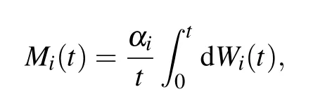


4.Stationary distribution


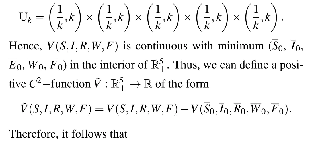


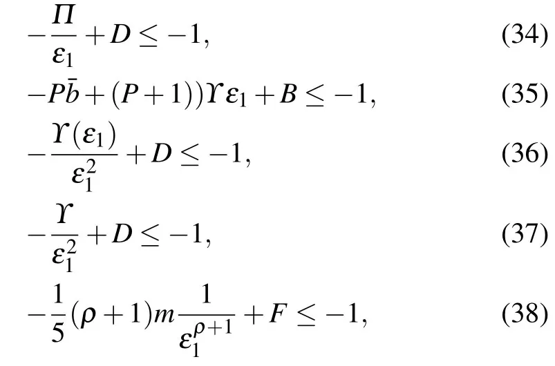




5.Investigation of the stochastic optimal control


6.Numerical simulations and discussion

6.1.Stochastic stability and numerical simulations


6.2.Numerical results on the stochastic control theory
7.Conclusion and directions
- Chinese Physics B的其它文章
- High sensitivity plasmonic temperature sensor based on a side-polished photonic crystal fiber
- Digital synthesis of programmable photonic integrated circuits
- Non-Rayleigh photon statistics of superbunching pseudothermal light
- Refractive index sensing of double Fano resonance excited by nano-cube array coupled with multilayer all-dielectric film
- A novel polarization converter based on the band-stop frequency selective surface
- Effects of pulse energy ratios on plasma characteristics of dual-pulse fiber-optic laser-induced breakdown spectroscopy

