A multi-channel approach for automatic microseismic event association using RANSAC-based Arrival Time Event Clustering (RATEC)

Lijun Zhu ,Lindsy Chung ,Jmes H.McClelln ,Ento Liu ,Zhigng Peng

a School of Electrical and Computer Engineering (ECE) at Georgia Institute of Technology,USA

b School of Earth and Atmospheric Sciences (EAS) at Georgia Institute of Technology,USA

Keywords:RANSAC Phase association Passive seismic Sensor array Classification Multi-channel

ABSTRACT In the presence of background noise,arrival times picked from a surface microseismic data set usually include a number of false picks that can lead to uncertainty in location estimation.To eliminate false picks and improve the accuracy of location estimates,we develop an association algorithm termed RANSAC-based Arrival Time Event Clustering (RATEC) that clusters picked arrival times into event groups based on random sampling and fitting moveout curves that approximate hyperbolas.Arrival times far from the fitted hyperbolas are classified as false picks and removed from the data set prior to location estimation.Simulations of synthetic data for a 1-D linear array show that RATEC is robust under different noise conditions and generally applicable to various types of subsurface structures.By generalizing the underlying moveout model,RATEC is extended to the case of a 2-D surface monitoring array.The effectiveness of event location for the 2-D case is demonstrated using a data set collected by the 5200-element dense Long Beach array.The obtained results suggest that RATEC is effective in removing false picks and hence can be used for phase association before location estimates.

1.Introduction

Microseismic event monitoring is an important tool in understanding the dynamic state of subsurface structure during hydraulic fracturing operation.The source mechanisms and locations of these microearthquakes can help characterize geometries and spatio-temporal evolution of fractures generated during fluid injections.Microseismic events are typically at low magnitudes and occur closely in space and time,presenting significant challenges for phase picking,association and event location(Eaton,2018).After initial phase picking,locating earthquakes involves two folds of operations:phase association and location estimation.The former refers to the procedure where a set of seismic phases are grouped into a common source,and the latter refers to solving for earthquake locations given a set of phases.Although less attention had been put on phase association in the past,it is now becoming a significant problem due to the recent improvement of detection abilities on weak seismic phases,mostly with deep-learning techniques(Ross et al.,2018;Zhu et al.,2019;Mousavi et al.,2020).

In global seismology,the association problem has been formulated as variants of statistical problems and solved by grid-search(Le Bras et al.,1994;Rodi and Toksoz,2000;Draelos et al.,2015).These algorithms search for the best grid that can maximize the coherency of observed and predicted arrival times.Formulation of such type can be categorized as the back-projection method(Kiser and Ishii,2017).At regional and local distances,sophisticated workflows based on back-projection or a grid-search algorithm have been created in order to meet different monitoring needs,e.g.,Earthworm,SeisCompP3,GLASS3,REAL,(Yeck et al.,2020;Zhang et al.,2019).More recently Ross et al.(2019)developed a deep-learning-based framework to solve association problems via modeling the temporal and contextual relationships of seismic phases.McBrearty et al.(2019) utilized graph theory to solve for phase association and source location simultaneously for area-specific back--projection problems.A reliable phase association result is the foundation of an accurate event location estimate.

Various earthquake location methods are implemented as standard procedures in data process pipelines.In earthquake seismology,the common practice is to use geometric methods(i.e.,triangulation)based upon direct arrivals picked at individual receivers (Zhang and Thurber,2003).Such a method is simple and only requires low computational cost,but it is only viable for borehole data(Maxwell et al.,2010) as arrivals detected on traces from surface data are less reliable when signal-to-noise ratios (SNR) are low (Duncan and Eisner,2010).Alternatively,semblance-based methods have been developed that do not rely on picked arrival times.These methods utilize semblance measures that involve stacking waveforms according to forward calculated travel times(Duncan,2005;Lakings et al.,2006;Tan et al.,2014;Stanˇek et al.,2015).In order to find the optimal location which yields the best stacking results,these methods have to discretize a monitoring region and then perform a grid search,which demands high computational resources.Although attempts have been made to accelerate the exhaustive search for the best location by global optimization such as differential evolution(Zhu et al.,2015) and particle swarm (Luu et al.,2016),these methods are,in general,slow on large monitoring regions with high spatial resolution requirements.Another set of methods use reverse time migration(RTM) to find event locations (Gajewski and Tessmer,2005;Artman et al.,2010;Nakata and Beroza,2016).These methods take advantage of waveform redundancies existing among receivers,and backward propagate wavefields to the source location in space and time through assumed models.The optimal locations are defined at the points where the energies are most focused.Recent development of full-waveform inversion (FWI) has inspired full-wave based methods (Witten and Shragge,2016;Sharan et al.,2016).However,like the RTM based methods,the finite-difference (FD) modeling they rely on is computationally intensive and can be slower than the grid search program in travel-time based methods.

The recent development of hydraulic fracturing produces increasing amounts of data from passive monitoring,which in turn demands a more efficient processing scheme for surface arrays that can be deployed without drilling monitoring wells.A recent study by Akram and Eaton(2016)summarized and compared the most common arrival time picking methods on a single trace,such as short-term over long-term average ratio (STA/LTA) (Allen,1978;Earle and Shearer,1994),a modified energy ratio(MER)(Han et al.,2009),a modified form of Coppens'method(MCM) (Sabbione and Velis,2010),and Akaike's information criterion(AIC)(Takanami and Kitagawa,1991),to name a few.A common theme in all of these methods is the use of processing to increase the significance of detected peaks and minimize the number of false picks from noisy data recorded by surface arrays,which leads to bad event location estimation.Ideally,when all the picks are perfect,a moveout curve can be computed to fit exactly through the arrival-time picks.Alternatively,Zhu et al.(2016) took advantage of the fact that a group of receivers with both good and bad picks still contains a subset of picks that follow an expected trend of arrival times when events are present.By fitting a moveout curve through subsets of picked arrival times using random sample consensus(RANSAC) (Fischler and Bolles,1981),Zhu et al.(2016) were able to recover the true arrivals in the presence of a large amount of false picks under low SNR conditions.

In this paper,we continue the study of applying RANSAC for picked arrival times and improve our method described in(Zhu et al.,2016)for realistic seismic monitoring scenarios.To reduce the false picks in time picking results and thus improve phase association and event location estimation,we propose a RANSAC-based arrival time clustering(RATEC)method as a pre-processing step that groups true picked times into different events and identifies false picks.A similar approach has recently been used to solve the phase association problem in Chile (Woollam et al.,2020).The primary difference between our RATEC method and other classic methods such as GA,GLASS3(e.g.,Le Bras et al.,1994;Yeck et al.,2020)is that we focus primarily on local scale,while the rest focus primarily on global scale or a combination of global,region and local scales.To demonstrate the accuracy of RATEC for 1-D receiver arrays,synthetic simulations are conducted in homogeneous,layered and non-layered isotropic media.The proposed scheme is also validated through a natural earthquake dataset collected on a 5200-element 2-D surface network in Long Beach,CA.All cases show that the RATEC framework is accurate and robust under low SNR conditions and applicable to a variety of different monitoring setups.

2.Motivation

To eliminate false picks generated by a time picking algorithm due to background noise,a classifier for true event picks is necessary.Such a classifier needs to learn the pattern of a seismic event from all arrivaltime picks and apply a rule to cluster the picks into two groups:true event and false picks.It also needs to be robust enough to accommodate the variety of patterns shown by different events.Since the true firstarrival times of any isolated seismic event result in a predictable moveout curve on a monitoring receiver array,a parametric model for valid moveouts can be used to build a classifier for true picks of an actual seismic event.

Moveout curves have been studied extensively in seismology by Dix(1955) and Dellinger et al.(1993) (See Appendix A).For homogeneous media,it is simply a hyperbola.Dix(1955)proved that moveout curves can also be modeled as hyperbolas for isotropic layered media when the receivers have small offsets relative to an event epicenter.He also gave explicit parametric equations for such curves (as a rotated hyperbola)when a tilting layer is present.Dellinger et al.(1993) showed that for transverse isotropic(TI)media,an elliptic parametric model can be used to approximate the expected moveout curves.Since horizontal variation in velocity is relatively small in microseismic monitoring,a hyperbola can be used to approximate the arrival time moveout curve for an event in non-layered media as well.To sum up,for a surface monitoring receiver array in microseismic monitoring,a quadratic parametric model exists for a moveout curve observed on a receiver array from a valid seismic event.Thus,the problem of finding the true picks for a seismic event can be solved by fitting a parametric model using picked arrival times.For simplicity,we only consider isotropic media with short offsets in this study,which corresponds to a hyperbola.Ellipses share the same quadratic model as hyperbolas,but with different parameter requirements.

However,due to poor SNR on surface monitoring arrays,there are many false picks that are far from true event moveout curves which we refer to as outliers.Curve fitting like least squares uses as many data points as possible to minimize the amount of misfit error.Although it is the optimal solution under a Gaussian random noise assumption,it fails dramatically in the presence of outliers which are unlikely to be Gaussian distributed.We,instead,adopt a random sampling scheme that repeatedly uses a minimum number of data points to fit a curve,and selects the best curve (hypothesized model) as the one with the most data points close to it,i.e.,with the maximum number of inliers.

This random sampling scheme was first proposed by Fischler and Bolles(1981)as random sample consensus RANSAC and then improved by many others (Stewart,1995;Torr and Zisserman,2000;Chum and Matas,2002,2005;Tordoff and Murray,2005).It has also been extended to fit multiple models simultaneously(Wang and Suter,2004;Toldo and Fusiello,2008).Based on the fitted hyperbolic model,the picked arrival times are,in fact,clustered into event groups and non-event groups.Such clustering not only separates picked arrival times into different phases,e.g.,P-wave and S-wave phases,but also improves the accuracy of subsequent source-location estimates by eliminating false picks due to noise.

3.Method

3.1.RANSAC overview

Despite many variations and adaptations of RANSAC (Choi et al.,2009),there are essentially two steps per iteration(hypothesize-and-test)

which will be repeated to yield the best fit to the data:

●Hypothesize:Aminimalsample subset (MinSet,denoted as) is randomly selected from the dataset and theuniquemodel parameters(pk) are computed for

●Test:Elements in the dataset (ΩD) are evaluated to determine which ones can be labeled asinliers,i.e.,consistent with the hypothesized model in the sense that the distance from the model's moveout curve is less than some prescribed value (δ).The set of all such inliers is called a consensus set (ConSet,denoted as

Notice that each RANSAC iteration requires very little computation and there exists a unique solution for each chosen MinSet.In this way,we can afford using a large number of iterations consistently to perfect a hypothesized model.Fischler and Bolles(1981)give a statistical analysis of the required number of iterations for the RANSAC process with an inlier ratio ofu(ratio between number of inliers and total number of data points).The number of iterations ˆNto guarantee that at least one ΩMwill only contain true picks with probabilitypis

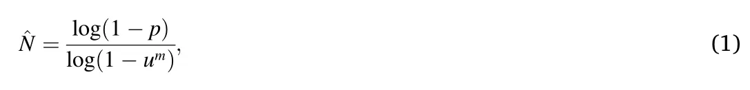
wheremis the size of a MinSet,which is 5 for a hyperbola and 9 for a hyperboloid.For example,when 50%of all picks are close to a hyperbola(u=0.5,m=5),we can guarantee a 99%chance of finding an outlierfree ΩM(p=0.99),if we run=145 iterations.For a 2-D surface array,m=9,and then=2356.Althoughmay be large,the core operations of deriving the hyperbola parameters and testing its validity are extremely fast so thousands of trials are reasonable.

The RANSAC process is summarized as the flow chart in Fig.1.After thekth iteration,the current best ConSetis updated with thekth ConSet ifhas more inliers.Thenis used to estimate the current best inlier ratiou＊.Based on equation(1),the number of iterations required ˆNcan be updated (Tordoff and Murray,2005).The currentis also compared against preset minimum and maximum valuesNmaxandNmin.Once the termination condition is satisfied,the best ConSetand model parameterp＊ will be returned;otherwise,the iteration loop will continue.

Fig.1. Flow chart of RANSAC process within each iteration.After many iterations the case with the biggest ConSet is declared the best parameter vector p＊.

3.2.Parameter estimation

The proposed method uses a quadratic model to estimate the parameters of a hyperbolic curve,which takes the following form:

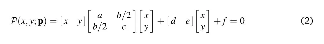
or,equivalently,

wherephas six real elements θ=(a,…,f),but there are actually only five free parameters,since one of the nonzero elements can be always normalized to 1.

We need to check two determinants in the QC process to guarantee that the quadratic form is a non-degenerate hyperbola.First,when the determinant

is nonzero(Δ1/=0),Equa(3)defines a non-degenerate conic section.To verify it is hyperbola,we must then check a second determinant

when Δ2>0,equation(3)defines a hyperbola.

Given a set ofnarrival time picks,(xi,yi)fori=1,…,n,we form then×6 data matrixDnand a 6×1 coefficient vectorp,such thatDnpis the model P(x,y;p) in (3) evaluated at the time picks.With measurement error,there will be a nonzero residualras follows:

We use only five picks to uniquely determinepas discussed previously.If all picks in ΩMare true picks,the residual termris usually negligible.Then we solve the linear systemD5p=0,which is effectively finding the null space ofD5.From the singular value decomposition(SVD) ofD5,it is easy to see that the last right singular vectorv6∊null(D5).Comparing with the pseudo-inverse method used in (Zhu et al.,2016),the solutionv6adopted here is not guaranteed to have the minimalL2norm.However,the SVD approach avoids numerical stability problems when the matrixis ill-conditioned.To process the large number of candidate MinSets ΩMefficiently,we do a quality control(QC)ofpby checking determinants,Δ1/=0 and Δ2>0,before proceeding to the more computationally demanding test step that computes the distance between the entire set of picks ΩDand the hypothesized RANSAC model to obtain a ConSet Ωc.

3.3.Add perturbation to MinSets

With the presence of measurement noise,the null-space method has a tendency to fit the wrong type of curve,namely a parabola or an ellipse,which is then eliminated by the parameter QC step.In noisy cases when the percentage of inliers is low,this problem may cause RANSAC to select a suboptimal parameter vector whose curve passes through some outliers as well as true inliers,as shown in Fig.2a.

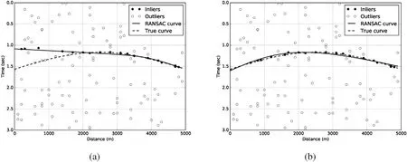
Fig.2. RANSAC classification of noisy data:(a) suboptimal fitting results from direct null space method,(b) optimal fitting results from null space method with perturbations.

To overcome this tendency when fitting quadratic models,a constrained least squares approach (Fitzgibbon et al.,1999;O'Leary and Zsombor-Murray,2004)has been developed to force the fitted curves to be hyperbolas (and ellipses) by solving a generalized eigen system determined by a constraint matrix.Although this method works for general hyperbolic curve fitting problems,its strategy runs counter to RANSAC's MinSet assumption,i.e.,using a random set with the minimum number of points.Least squares employs as many data points as possible in order to minimize the distance between the data and the optimal model.However,the more points required in the MinSet,the smaller the possibility that a MinSet will be outlier-free.This dilemma restricts the ability of the constrained least-squares method to find a proper model when the SNR is low.

Fortunately,the RANSAC process has the luxury of running a very large number of fast iterations to find the optimal model.By randomly perturbing the time picks into produce a few additional MinSets and running more iterations,we can combat the effects of measurement noise.For example,after adding a small perturbation to the picked arrival time in Fig.2a,the correct moveout curve is selected in Fig.2b.Although we perturbed the picked arrival times to get the model coefficients,the final output of inliers and the location estimation are conducted on the original“unperturbed”data.

3.4.Processing pipeline

The overall processing pipeline of RATEC is summarized in Fig.3.Arrival times are picked on pre-processed data to extract event features out of seismic traces as time pick pairs (x,t).In this study,we use the widely adopted short-term over long-term average ratio (STA/LTA)method to generate a characteristic function for each seismic trace.However,any valid time picking method,such as those included in(Akram and Eaton,2016),can replace STA/LTA depending on the specific SNR condition.Peak detection is conducted on characteristic functions to generate (x,t) pairs which are then clustered by RANSAC to select true picks that correspond to a valid event moveout.These clustered picks can be fed into other location estimation programs such as double difference(Waldhauser and Ellsworth,2000;Zhang and Thurber,2003).When no prior knowledge of the velocity model is available,we provide a moveout curve fitting based event location estimator assuming a homogeneous medium.

Fig.3. Processing pipeline of proposed RATEC method:peak detection can be customized to adapt to the RANSAC framework;classification based on RANSAC eliminates false picks when estimating the moveout curve for an event.

Notice that this is a highly flexible framework in which multiple methods can be used for each block to optimize the performance for different datasets.Fig.3 provides a generic approach to demonstrate the accuracy and robustness of RATEC;however,it can be customized to specific needs and easily incorporated into any time picking based processing workflow.

4.Pre-process seismic data for RANSAC classification

The input data can be pre-processed to facilitate peak detection and help RANSAC better fit the moveout curve.The strategy is to encourage more time peaks by including as many weak events as possible while not introducing too many false picks.Here we give an example preprocessing method that takes advantage of RANSAC's ability to eliminate outliers while including more weak picks that might be related to a true event.

4.1.Guided peak detector

A straightforward approach to peak detection in characteristic functions is to find the global maximum on each trace.However,such peak locations can easily be affected by background noise as shown in Fig.4a,and smaller events are overlooked when multiple events are present.Likewise,locating peaks by local maxima is adversely affected by background noise since a noise signal tends to have a large number of local peaks.

One way to include more time picks is to use thresholding at a fraction of the maximum value.Shown in Fig.4b,setting the threshold to 70%of the maximum value yields more picks.This method succeeds in finding more arrival times(both true and false),but puts a heavy burden on the following classification block if too many of these peaks are false ones.A better way to include more time picks is to make a rough estimate of where the real signal lies based on a signal attribute such as the local zero-crossing rate defined below:

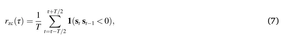
where1(stst-1<0) counts sign changes inst=sgn(s(t)),andTis the interval over whichrzc(τ) is computed.The local zero-crossing rate should be low when the signal is present.Using 95% of the global maximum threshold on the characteristic function weighted byFig.4c shows that this guided peak detector successfully picks only the real arrival time peak and the global maximum (due to severe background noise).

4.2.Merging close picks

With background random noise,there may be multiple peaks clustered around a true event pick.This not only leads to more computational cost in later location algorithms but also introduces uncertainty into event locations.Such a problem can be solved by merging close picks into one pick.A common practice in manual picking is to use the starting point of a pick cluster as the event arrival time.This is reasonable as the peak detector usually picks both the arrival signal (first break) and its coda wave (points that follow which form a cluster of time picks).However,it not only requires more computation to search for closely located peaks but also can be misled by a false pick that slightly leads the true picks.It can soon become tricky to set the correct parameter for how close the picks need to be to each other for a merge.

We consider using Gaussian smoothing which is widely used for edge detection in image processing(Basu,2002).Gaussian smoothing helps in reducing details(adjacent small peaks)within the characteristic function and attenuating insignificant local peaks due to noise.It convolves the response function with a Gaussian function defined below:

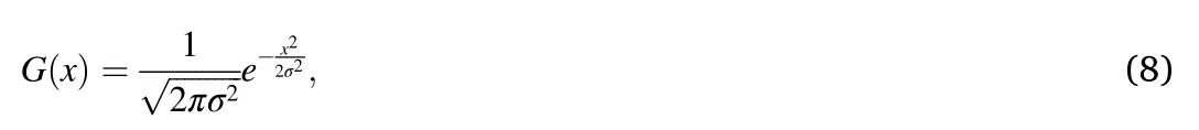
where σ is the standard deviation which can be set as the dominant duration of a wavelet (0.1 s in this case).Although Gaussian smoothing cannot eliminate all the close false picks,it can help mitigate such errors.Note that Gaussian smoothing is only helpful for traditional phase picking methods,e.g.STA/LTA,which are sensitive to local peaks.It should be omitted when using phase picking method based on full waveforms,such as cross-correlation (Song et al.,2010) or neural networks (Zhu et al.,2019).

5.Seismic examples

In this section,we explore the performance of the proposed RATEC method in a more realistic scenario of seismic processing.In the first example,a Ricker wavelet is manually delayed with moveout from a homogeneous medium assumption to demonstrate the essence of the proposed method.The second example uses a recorded seismic trace consisting of P-wave and S-wave phases which are then manually delayed according to a layered velocity model to simulate data from an array.This is a typical scenario in microseismic surface monitoring and we demonstrate that RATEC is able to extract both P-wave and S-wave phases and group them into event clusters.In the third example,we explore the problem when the layered model assumption is violated by using the Marmousi2 velocity model to generate the testing data with a finite-difference time-domain (FDTD) simulation.In the final example,we demonstrate that RATEC can be easily extended to the case of a 2-D surface monitoring array by validating it on a 5200-element 2-D dense array deployed for earthquake monitoring in Long Beach,CA.

5.1.Ricker wavelet in homogeneous media

For Fig.5a,a 25-element linear array with nominal spacing of 200 m is deployed on the surface(i.e.,5 km aperture)to monitor a deep event 2 km below the array center.The receiver locations are perturbed by additive white Gaussian noise (AWGN) with σ=50 m to simulate receiver offsets in the field away from uniformly spaced locations due to unavoidable physical restrictions in the field.Note that such perturbations effectively create a nonuniform linear array.The raw data section is shown in Fig.5a with the true moveout curve marked with a blue dashed line.

The source wavelet employed here is a Ricker wavelet,and the medium is assumed to be homogeneous with a velocity of 3 km/s.AWGN with peak signal-to-noise ratio (PSNR) of 6 dB is added to simulate random background noise.Because PSNR is not affected by the trace length,it is used to measure the noise level throughout the paper.Its definition is as follows:

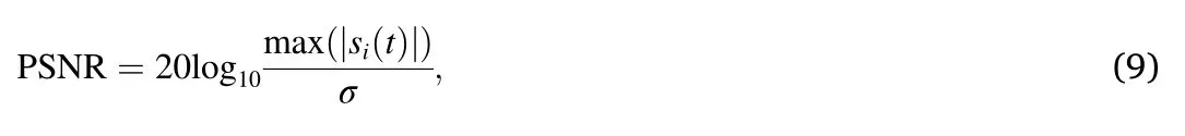
wheresi(t)is the signal at theith receiver,and σ is the standard deviation of the AWGN.

After applying the STA/LTA method on each trace,we use the zerocrossing guided peak detector and peak merging to find the candidate arrival time picks.These picks are passed to a classification block to be grouped into event (inlier) and non-event (outlier) clusters.When zoomed in around the moveout curve as shown in Fig.5b,a small deviation between the fitted curve and the true moveout curve is observed;however,all picks close to the true moveout curve are successfully clustered into the event/inlier group.

Fig.4. Detection methods for single event case on noise trace with PSNR=6 dB (true peak at t=1.0 s):(a) global maximum;(b) thresholding at 70% of global maximum;and (c) adaptive thresholding at 95% of global maximum weighted by the local zero-crossing rate.Adaptive thresholding picks true arrival time cluster with only one false pick.

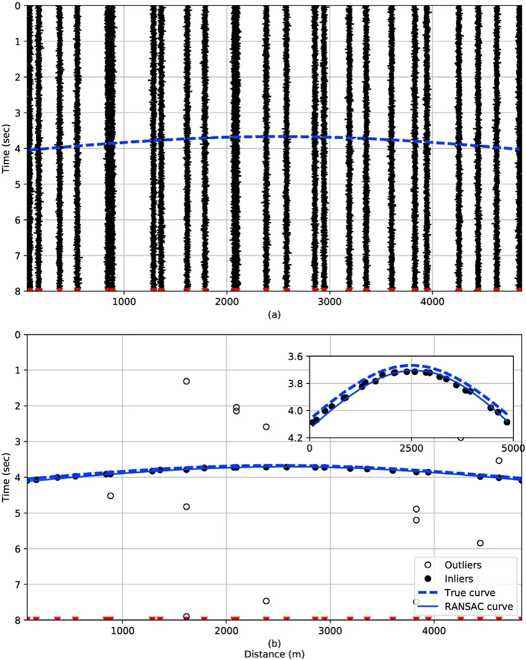
Fig.5. Simple example of time picking:(a) raw traces of a 25-element nonuniform linear array with an aperture of 5 km.Source waveform is a Ricker wavelet of 10 Hz central frequency and the PSNR=6 dB.Blue dashed curve indicates the true moveout.(b) Arrival times picked on each trace clustered into inlier (solid dots) and outlier (empty dots) groups.Insert in the top right shows a zoomed-in view along the vertical (time) axis.

Once clustering and correction are complete in the previous steps,the improved picked arrival times in this example can be used to locate events.There are many existing event location methods that use picked arrival times,such as Geiger's method (Geiger,1912) and the double-difference method(Waldhauser and Ellsworth,2000;Zhang and Thurber,2003).The corrected arrival times can be used by these methods with known velocity models to improve the location estimation.

When the velocity model is unknown,we can assume a homogeneous medium in order to compute predicted arrival times from possible source locations.Based on the inliers given by RATEC,we can minimize a nonlinear objective function that measures the sum of squared errors between the RATEC classified inlier picks and the predicted arrival times

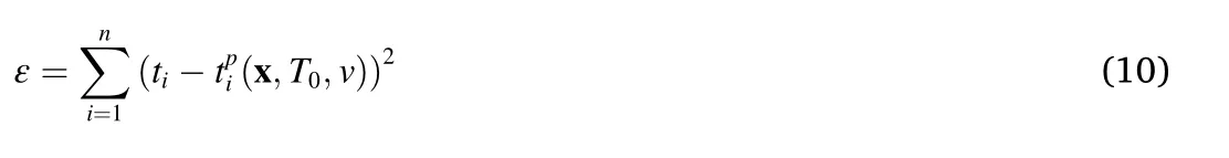
wheretiis the RATEC pick at theith receiver andis the predicted arrival time which is a hyperbola that depends on the event locationx,origin timeT0,and homogeneous velocityv.The minimizer of Equa.(10)gives the event location and event origin time,and the medium velocity simultaneously.

To validate the accuracy of this location scheme,1 000 Monte Carlo experiments are conducted to compare the results with and without the RATEC scheme under different noise levels.Only the first 100 data points,which is sufficient to capture the location estimation distribution as a point cloud,are shown in Fig.6 to avoid crowding.For low background noise,PSNR=20 dB,both methods obtain the event location accurately around the true event location(2 500,2 000)m as shown in Fig.6a.The uncertainty in depth is mostly a result of the array geometry which has poor resolution in the direction perpendicular to the linear array.The location results with RATEC have a more compact distribution around the true location.There are more blue dots than yellow triangles within the one-sigma confidence interval indicated by the blue ellipse.The location estimates without RATEC start to fall apart when the PSNR is around 8 dB as shown in Fig.6b.Although most of the yellow triangles are still around the true location region with a larger spread,there are a significant number of location estimates far away from the event region.On the other hand,the results with RATEC show a consistent distribution around the true event region in Fig.6b.Under severe noise as shown previously in Fig.5 with 7 dB PSNR,the location results without RATEC become completely unreliable while those with RATEC still give very good estimates.In Fig.6c about 50%of the blue dots,but only one yellow triangle,lie within the confidence ellipse.

The accuracy of the location estimate with and without RATEC measured in root-mean-square error (RMSE) for the complete 1 000 Monte Carlo experiments are shown in Table 1.With the RATEC correction,the location estimate in easting is improved significantly.The error in depth is much larger but is reduced by applying the RATEC correction.

Table 2 Parameters used in all simulations.

Fig.6. Location results with and without the RATEC scheme using 100 Monte Carlo experiments under three different background PSNR noise levels:(a)20 dB,(b) 8 dB,and (c) 6 dB.Blue ellipses (in the insets) show the one-sigma confidence interval of the event location estimator.Note the changing axis limits for the insets.The red star indicates the minimizer for the noiseless case which overlaps the true event location at (2 500,2 000) m.

Table 1 RMSE of RATEC location results from 1000 Monte Carlo experiments.

5.2.Recorded seismic trace in layered model

Here,the seismic trace shown in Fig.7a is used as a source signal.After manually picking the P-wave and S-wave phases,shown in Fig.7b and c respectively,the P and S phases are delayed separately according to their travel time (T) computed from a layered model against horizontal offset(x)using the parametric Equa.(11)given by Dix(1955).A detailed explanation can be found in Appendix A.

wherepis the ray parameter that is constant among all layers,hkandvkare layer thickness and layer velocity which defines a layered velocity model.Unlike the hyperbolic approximation discussed before,this equation is mathematically valid even whenx→∞;however,the direct wave may not necessarily be the first arrival wave whenxis large.In addition,for largexcases,the SNR condition may be too bad for a valid location problem.Thus,all examples here are conducted for smallx(less than 5 km).

The layered velocity model used in this example as shown in Fig.8a is taken from Marmousi2 elastic velocity model (Martin et al.,2006).The top water layer in Marmousi2 is removed and event source is located around 2.5 km deep.The same nonuniform surface array as in Section 5.1 is used for monitoring underground seismic events occurring at the center of the array.

With noise at 10 dB PSNR,the P-wave and S-wave arrivals are not obvious in the raw data shown in Fig.8b.With a spectrogram the dominant frequency of the arrival event is estimated to be 10 Hz,so a low-pass filter with cutoff frequency at 20 Hz is used as pre-processing.Both P-wave and S-wave arrivals are observed in Fig.8c after low-pass filtering.The result of applying the RATEC method is shown in Fig.8d,where moveout curves were generated by fitting the classified and corrected arrival time picks.The proposed method is used iteratively in this example to extract all possible event phases:after one moveout curve is detected and identified,its outliers are used as the input for the next iteration to search for more curves until there are not enough time picks to successfully define a moveout curve.Here,both P-wave(blue)and Swave(green)phases are identified in this example with most of the true arrival times labeled correctly.

5.3.Ricker wavelet in non-layered media example

Although RATEC is based on a layered velocity model assumption,it is robust enough to handle non-layered models to some extent.In Fig.9a,the acoustic Marmousi model is used to introduce horizontal variation in the velocity model.A finite-difference time-domain based numerical simulation is used to generate the surface receiver data shown in Fig.9b with 10 dB PSNR of AWGN.Since each trace has different peak value,which is common in a real seismic scenario,the PSNR defined here uses the global peak of all the traces.Receivers in the layered region (0-1 000 m horizontally) tend to have better SNR than those in the nonlayered region(1 000-1 500 m).

After applying the RATEC scheme,Fig.9c shows the results of curve prediction and arrival time labels.Even though the true moveout is not exactly a hyperbola,the RATEC method is able to label all the true arrival times given a 0.05 s tolerance range.Zoomed in around the layered region,good prediction and perfect labeling are observed in Fig.9d.Notice that there now exists larger offsets between picked and true arrival times.Fig.9e shows the results in the non-layered region where the SNR is worse.Despite the fact that many picks in that region are false picks,RANSAC is able to eliminate most of the picks far away from the true moveout curve and label the true time picks correctly.

5.4.Surface extension on microearthquake data

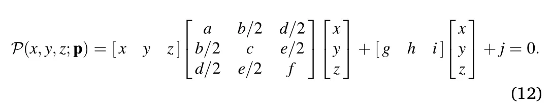
RATEC can be easily extended to a surface array by changing the underlying hyperbolic curve model to a hyperboloid surface model.Similar to Equa.(2),a hyperboloid surface can be defined using a 3D quadratic equation with ten parameters which takes the following general form:

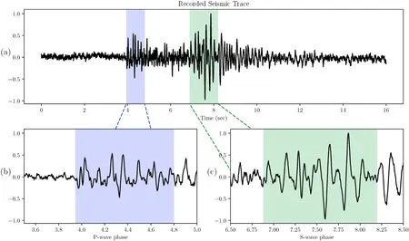
Fig.7. (a) Recorded seismic trace with P-wave (blue) and S-wave (green) phases for layered model simulation,(b) manual pick of P-wave phase,and (c) S-wave phase.The phase picks are the beginning of the marked time windows.

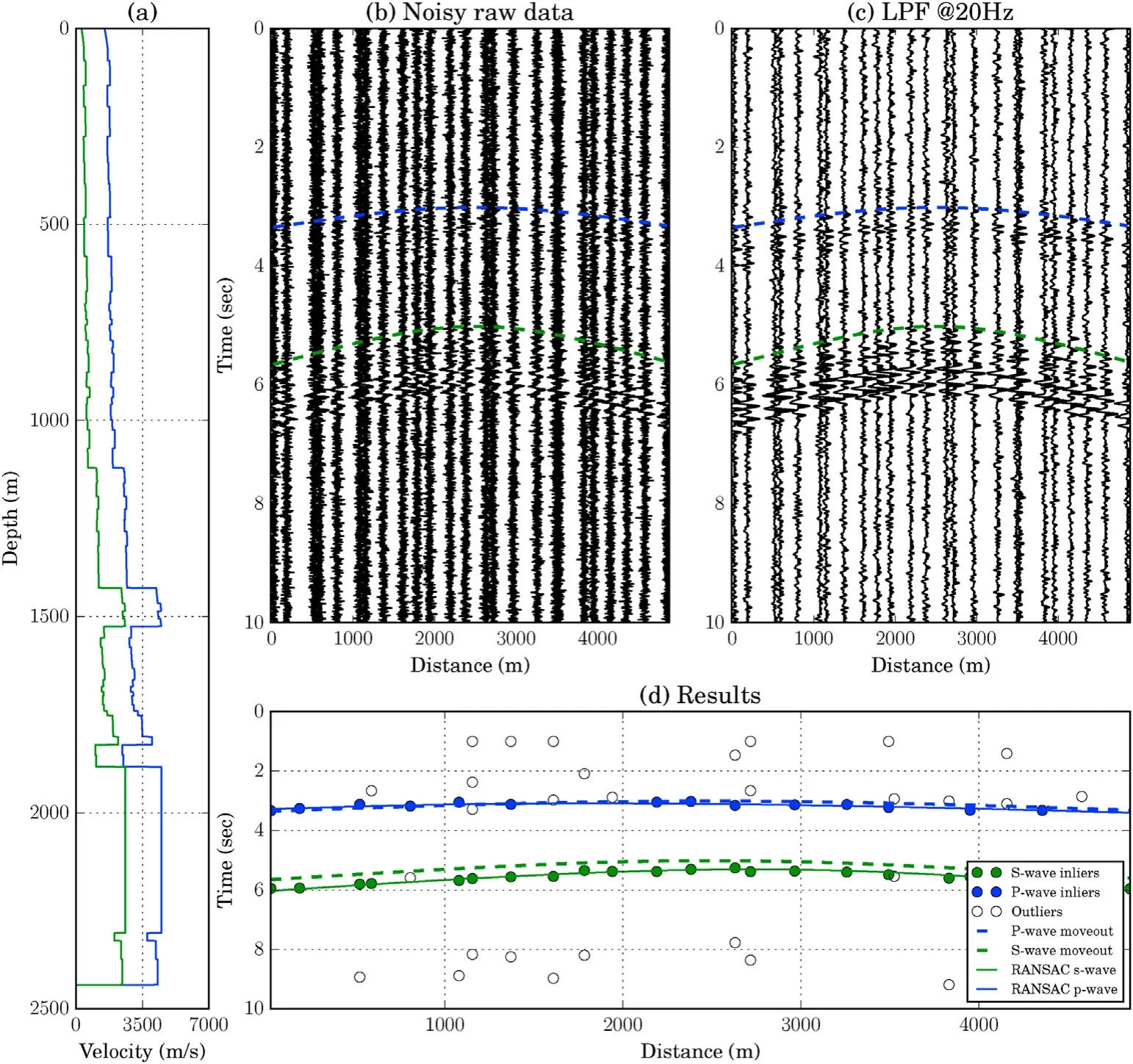
Fig.8. Layered velocity model example using recorded seismic trace with P-wave and S-wave phases:(a)1-D velocity model from Marmousi2;(b)noisy raw data with PSNR=10 dB with respect to the S-wave peak;(c) 20 Hz low-passed data;(d) fitted moveout curve and classification results comparing to true P-wave and S-wave moveout curves.

Fig.9. Marmousi model example under 10 dB PSNR:(a)velocity model(red dot indicates source location),(b)synthetic data(red line indicates true arrival times),(c)RATEC results shown as solid line versus true arrivals shown as dashed line,(d) zoomed-in results between 400 m and 600 m and (e) zoomed-in results between 1 000 m and 1 200 m.

Using the same RATEC scheme,we can adapt the framework to hyperboloid surface fitting by finding the parameter vectorp=(a,b,…,j)in a 10-dimensional space.Although this may seem to be a much larger parameter space,it adds little burden on the search process as RANSAC searches only ΩMrather than complete parameter space.

The proposed method was then tested on a data set of 50 s collected by the Long Beach nodal array in southern California which contains 5 200 sensors.The top view of the sensor array is shown in Fig.10.Prior to applying the RATEC scheme,no reliable location estimation can be given by picked arrival times due to a large number of false picks as shown in Fig.11.After applying RATEC,the best-fitted hyperboloid surface from 3D RATEC is shown as the red surface.On a laptop,it takes just 31 s to finish this classification process,which is sufficient for real-time processing (note that the recording duration is 50 s).At this point,we can use the RATEC picked arrival times to locate an event,but we must use a homogeneous medium assumption since there is no velocity model known prior to this experiment.Based on the true picks classified by RATEC,this seismic event is recognized as a surface event whose location is shown by its epicenter marked by the red star in Fig.10.In order to verify our result,we schematically show the corresponding raw-data snapshot on the sensor array in Fig.11.The gray-scale of the dots indicates the clipped signal amplitude on the corresponding sensor.The red circle in Fig.11 confirms that in the inverted time and location using the classified true picks,there is indeed a weak event that is barely visible in the array.Moreover,the work log shows that there is a surface source in the estimated area but the local earthquake catalog has no record of earthquakes during the event time.In Fig.12 we show the time picking results that contain a large number of false picks.The best-fitted hyperboloid surface from 3-D RATEC is shown as the red surface.

Fig.10. Top view of the sensor array with located event indicated by red star.

Fig.11. Snapshot of the seismic dataset at time t=3 020.00 s;the visible event lies inside the red circle.

5.5.Parameter selection

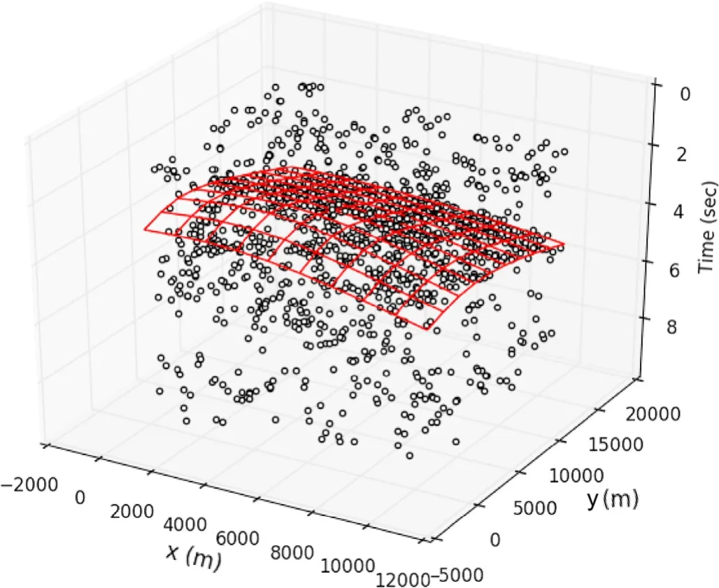
Fig.12. Top view of the picks (◦) from the 2D sensor array with fitted surface in red.

Although it may seem that there are many parameters to be set for the RATEC method,they are actually tied to just one parameter that can be estimated from the data itself:fdom,the dominant frequency of the source wavelet.All parameters used in the above simulation examples are summarized in Table 2 and their recommended relationship tofdomis listed as well.Cut-off frequency is chosen as the Nyquist frequency forfdom.Half period or wavelength is commonly used in signal detection and thus is chosen as the STW and ThresDist.We follow the usual convention and choose LTW=10×STW.Zero-crossing rate measures the long-term effects of the signal so we choose the same window length as LTW.Gaussian smoothing tries to remove the short-term extreme values in the signal so we choose the same window as STW,0.5Tdom,which makes the smoothing window exactly the full wave period.The choice of additive noise sigma beingTdommakes the picked arrival time with noise lie in the waveform period with over 90% probability (two sigmas of the normal distribution).These parameters work well with the Ricker wavelet based simulations since the dominant frequency is a valid measurement of wavelet length(dominant periodTdom∝fdom).However,sometimes the true wavelet length is longer than the dominant period (Tdom),e.g.,a seismic trace with dispersion.In this case,we can fix the cut-off frequency at 20 Hz but makeTdomlonger to alleviate the problem.

6.Conclusion

In this paper,we tackled the problem of phase association and event location estimation from arrival times by fitting a parametric model and then proposed a RANSAC-based fitting method (RATEC) to classify picked arrival times and detect possible events.RATEC discriminates true event arrival times from false picks by associating them with some reasonable moveout curves.Tests with synthetic data show that RATEC performs well for a 1-D linear array under layered medium assumption,as well for non-layered media and in the presence of dispersion.RATEC is also expandable to the case of 2-D surface arrays by replacing the underlying hyperbolic curve model with a hyperboloid surface model.The effectiveness of event location for the 2-D case is demonstrated in a 5200-element dense 2-D array for earthquake monitoring at Long Beach,CA.

In this study,we did not make any assumption on the seismic velocity in the study region.Knowing the average velocity or a 1-D velocity model can be helpful to constrain the curvature of the fitted hyperbolas.It is also possible to impose a constraint of P–S phase separation time to further improve the fidelity of the fitted curves.This is beyond the scope of this paper and will be discussed in a follow-up work.

Acknowledgement

This work is supported by the Center for Energy and Geo Processing at Georgia Tech and King Fahd University of Petroleum and Minerals.We are grateful to Zefeng Li for helpful discussions and the analysis of microearthquake data.The seismic data analyzed in this study are owned by Signal Hill Petroleum,Inc.and acquired by NodalSeismic LLC.We thank NodalSeismic LLC for making the one-week data available in this study.LYC and ZP are partially supported by NSF award EAR-1818611.

Appendix A.Parametric model of moveout curves

In many microseismic applications,accurate velocity models may not be available.However,a layered medium is commonly assumed for a shale rock region,in which case an estimate of the event location can be inferred from the arrival-time moveout curve across the monitoring geophone array.Using arrival times not only has a clear physical meaning but also it turns out to be computationally efficient.The primary requirement for this method to work is that there exists a parametric modelT(x)that approximates the arrival timeTversus horizontal offsetx.By estimating the finite number of model parameters,an event location can be uniquely determined.Over the years,such parametric models have been gradually updated and generalized for various types of media.

A.1 Homogeneous medium

For a homogeneous medium,the geometry of ray tracing is shown in Fig.13a.For an event originating at timeT0and location(x0,h),a sensor atxwill receive the signal at timeT(x),so the relation between source-to-receiver travel timeT(x)-T0and the horizontal offset (x-x0) is

where we note that the zero-offset travel time isT(x0)-T0=h/v.The travel-time equation(13)can be rewritten in a form that is recognizable as the standard form of a hyperbola

Thus,an event originating at timeT0and location(x0,v[T(x0)-T0])can be uniquely determined by estimating the parametersT0,x0,T(x0),andvin equation(13),or(14).The estimation involves fitting a hyperbola to the picked arrival timesT(xj) in a linear surface array.

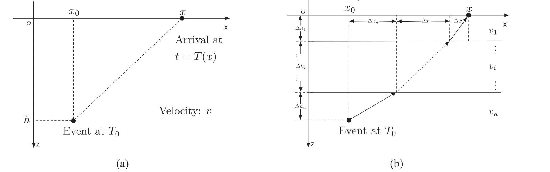
Fig.13. Geometry of ray paths and travel time for (a) homogeneous medium with velocity v,and (b) a layered media

A.2 Layered isotropic media

A layered isotropic media,shown schematically in Fig.13b,is a little more complex than a homogeneous medium.The travel time ΔTiand horizontal offset Δxiof thei-th layer can be modeled as follows:

wherep=sin θi/viis the ray parameter in Snell's law which is constant over all layers.Within each layer,the travel time has a hyperbolic relationship with offset,i.e.,ΔTi(xi) defines a hyperbola,so the overall travel time ΔT(x)=T(x) -T0computed as the sum is not exactly a hyperbola

However(Dix,1955),proved that a layered isotropic media behaves approximately like the homogeneous model when the offsetxis close to zero.In other words,a hyperbolic moveout curve is observed near Δx=0 for an isotropic layered model with an equivalent velocity of

In microseismic monitoring the receiving array is usually positioned over the top of the monitored events,so the offsetxshould be close to zero and the approximation(17)can be used.Moreover,Dix(1955)gave a correction for a tilted layered model as well—the(approximate)relationship betweenTandxis still described by a hyperbolic curve

where θ is the tilt angle.

A.3 Parametric model for TI media

It is the parametric model rather than a hyperbolic curve that is essential to the data fitting method we will propose.In cases of transverse isotropic(TI)media,Dellinger et al.(1993)gave an elliptic approximation of the arrival-time moveout curve

wherexis the offset,T(0)is the vertical travel time,VNMOis the near-offset NMO velocity,andFWis a dimensionless anisotropy parameter.Although equation (19) is a rational form with a fourth-order numerator and seems to be far from a hyperbolic curve,the basic idea is still valid:fitting a parametric model forT(x)to locate an event.In this paper,we use the simpler hyperbolic model as a demonstration.The method to be proposed can be extended easily to other types of parametric models that adapt to different types of media.