Learning Convex Optimization Models

Akshay Agrawal, Shane Barratt, and Stephen Boyd,

Abstract—A convex optimization model predicts an output from an input by solving a convex optimization problem. The class of convex optimization models is large, and includes as special cases many well-known models like linear and logistic regression. We propose a heuristic for learning the parameters in a convex optimization model given a dataset of input-output pairs,using recently developed methods for differentiating the solution of a convex optimization problem with respect to its parameters.We describe three general classes of convex optimization models,maximum a posteriori (MAP) models, utility maximization models, and agent models, and present a numerical experiment for each.

I. INTRODUCTION

A. Convex Optimization Models

A convex optimization model has the form

where the objective functionE:X×Y →R∪{+∞} is convex in its second argument, and θ ∈Θ is a parameter belonging to a set of allowable parameters Θ. The objective functionEis the model’senergy function, and the quantityE(x,y;θ) is the energy ofygivenx; the energyE(x,y;θ) can depend arbitrarily onxand θ, as long as it is convex iny. Infinite values ofEencode additional constraints on the prediction,sinceE(x,y;θ)=+∞ implies φ(x;θ)≠y. Evaluating a convex optimization model atxcorresponds to finding an outputy∈Y of minimum energy. The function φ is in general setvalued, since the convex optimization problem in (1) may have zero, one, or many solutions. Throughout this paper, we only consider the case where the argmin exists and is unique.

Convex optimization models are particularly well-suited for problems in which the outputsy∈Y are known to have structure. For example, if the outputs are probability mass functions, we can take Y to be the probability simplex; if they are sorted vectors, we can take Y to be the monotone cone; or if they are covariance matrices, we can take Y to be the set of symmetric positive semidefinite matrices. In all cases, convex optimization models provide an efficient way of searching over a structured set to produce predictions satisfying known priors.

Because convex optimization models can depend arbitrarily onxand θ, they are quite general. They include familiar models for regression and classification as specific instances,such as linear and logistic regression. In the basic examples of linear and logistic regression, the corresponding convex optimization models have analytical solutions. But in most cases, convex optimization models must be evaluated by iterating a numerical algorithm.

Learning a parametric model requires tuning the parameters to make good predictions on D and ultimately on held-out input-output pairs. In this paper, we present a gradient method for learning the parameters in a convex optimization model;this learning problem is in general non-convex, since the solution map of a convex optimization model is a complicated function. Our method uses the fact that the solution map is often differentiable, and its derivative can be computed efficiently, without differentiating through each step of the numerical solver [1]–[4].

We limit our attention to optimization models that are convex for three reasons: convex programs can be solved globally, efficiently, and reliably [5], which makes inference tractable; the solution map is often differentiable [1], [3],which makes learning tractable; and convex optimization models are general, since they can depend arbitrarily onxand θ(e.g., we can takeE(x,y;θ)=‖y-f(x,θ)‖2, wheref(x,θ) can be any function, such as a neural network).

Contributions:The contributions of our paper are the following:

1) We describe a new type of machine learning model, the convex optimization model, which makes it both possible and easy to express priors and enforce constraints on the model output.

2) We show how to fit convex optimization models using recently developed methods for differentiating through the solution map of convex programs.

3) We give several examples of convex optimization models, grouping the examples by application area, i.e., MAP inference, utility-maximizing processes, and agent models.We include numerical experiments showing how to use opensource software to fit these models.

Outline:Our learning method is presented in Section II for the general case. In the following three sections, we describe special cases of convex optimization models with particular forms or interpretations. In Section III, we interpret convex optimization models as solving a maximum a posteriori(MAP) inference task, and we give examples of these MAP models in regression, classification, and graphical models. In Section IV, we show how convex optimization models can be used to model utility-maximizing processes, and in Section V,we give examples of modeling agents using the framework of stochastic control. In Section VI, we present numerical experiments of learning convex optimization problems for a number of prediction tasks.

B. Related Work

Structured Prediction:Structured prediction refers to supervised learning problems where the output has known structure [6]. A common approach to structured prediction is energy-based models, which associate a scalar energy to each output, and select a value of the output that minimizes the energy, subject to constraints on the output [7]. Most energybased learning methods are learned by reducing the energy for input-output pairs in the training set and increasing it for other pairs [8]–[11]. More recently, the authors of [12], [13]proposed a method for end-to-end learning of energy networks by unrolled optimization. Indeed, a convex optimization model can be viewed as a form of energy-based learning where the energy function is convex in the output. For example, input-convex neural networks (ICNNs) [14] can be viewed as a convex optimization model where the energy function is an ICNN. We also note that several authors have proposed using structured prediction methods as the final layer of a deep neural network [15]–[17]; of particular note is[18], in which the authors used a second-order cone program(SOCP) as their final layer.

Inverse Optimization:Inverse optimization refers to the problem of recovering the structure or parameters of an optimization problem, given solutions to it [19], [20]. In general, inverse optimization is very difficult. One special case where it is tractable is when the optimization problem is a linear program and the loss function is convex in the parameters [19], and another is when the optimization problem is convex and the parameters enter in a certain way[21], [22]. This paper can be viewed as a heuristic method for inverse optimization for general convex optimization problems.

Differentiable Optimization:There has been significant recent interest in differentiating the solution maps of optimization problems; these differentiable solution maps are sometimes calledoptimization layers. Reference [23] showed how quadratic programs can be embedded as optimization layers in machine learning pipelines, by implicitly differentiating the KKT conditions (as in the early works [24],[25]). Recently, [2], [3] showed how to efficiently differentiate through convex cone programs by applying the implicit function theorem to a residual map introduced in [4],and [1] showed how to differentiate through convex optimization problems by an automatable reduction to convex cone programs; our method for learning convex optimization models builds on this recent work. Optimization layers have been used in many applications, including control [26]–[29],game-playing [30], [31], computer graphics [18], combinatorial tasks [32], automatic repair of optimization problems[33], and data fitting more generally [14], [34]–[36].Differentiable optimization for nonconvex problems is often performed numerically by differentiating each individual step of a numerical solver [37]–[40], although sometimes it is done implicitly; see, e.g., [26], [41], [42].

II. LEARNING CONVEX OPTIMIZATION MODELS

In this section we describe a general method for learning the parameter θ in a convex optimization model, given a data set consisting of input-output pairs (x1,y1),...,(xN,yN)∈X×Y.We letyˆi=φ(xi;θ) denote the prediction ofyibased onxi, fori=1,...,N. These predictions depend on θ, but we suppress this dependency to lighten the notation.

A. Learning Problem

The fidelity of a convex optimization model’s predictions is measured by a loss functionL:Y×Y →R. The valueL(yˆi,yi)is the loss for theith data point; the lower the loss, the better the prediction. Throughyˆi, this depends on the parameter θ. Our ultimate goal is to construct a model that generalizes, i.e., makes accurate predictions for input-output pairs not present in D. To this end, we first partition the data pair indices into two sets, a training set T ⊂{1,...,N} and a validation set V={1,...,N}T. We define the average training loss as

We fit the model by choosing θ to minimize the average training loss plus a regularizerR:Θ →R∪{∞}, i.e., solving the optimization problem

with variable θ. The regularizer measures how compatible θ is with prior knowledge, and we assume thatR(θ)=∞ for θ ∉Θ,i.e., the regularizer encodes the constraint θ ∈Θ. We describe below a gradient-based method to (approximately) solve the problem (2).

We can check how well a convex optimization model generalizes by computing its average loss on the validation set

In some cases, the model or learning procedure depends on parameters other than θ, called hyper-parameters. It is common to learn multiple models over a grid of hyperparameter values and use the model with the lowest validation loss.

B. A Gradient-Based Learning Method

In general, L is not convex, so we must resort to an approximate or heuristic method for learning the parameters.One could consider zeroth-order methods, e.g., evolutionary strategies [43], Bayesian optimization [44], or random search[45]. Instead, we use a first-order method, taking advantage of the fact that the convex optimization model is often differentiable in the parameter θ.

Differentiation:The output of a non-pathological convex optimization model is an implicit function of the inputxand the parameter θ. When some regularity conditions are satisfied, this implicit function is differentiable, and its derivative with respect to θ can often be computed in less time than is needed to compute the solution [2]. One generic way of differentiating through convex optimization problems involves a reduction to an equivalent convex cone program,and implicit differentiation of a residual map of the cone program [2]; this is the method we use in this paper. For readers interested in more details on the derivative computation, we suggest [1], [2], [4]. In our experience, it is unnecessary to check regularity conditions, since we and others have empirically observed that the derivative computation in [2] usually provides useful first-order information in the rare cases when the solution map is not differentiable at the current iterate [1], [29]. In this sense,convex optimization models are similar to other kinds of machine learning models, such as neural networks, which can be trained using gradient descent despite only being differentiable almost everywhere.

Learning Method:We propose a proximal stochastic gradient method. The method is iterative, starting with an initial parameterθ1.The firststepiniterationkis tochoosea batch of(training)datadenoted Bk⊂T. Thereare many ways to do this, e.g., by cycling through the training set or by selecting at random. The next step is to compute the gradient of the loss averaged over the batch

This step requires applying the chain rule for differentiation to |Bk| compositions of the convex optimization model(discussed above) and the loss function. The final step is to update θ by first taking a step in the negative gradient direction, and then applying the proximal operator ofR

wheretk＞0is a step size.We assumethattheproximal operator ofRis single-valued and easy to evaluate. WhenR(θ)is the {0,∞} indicator function of Θ, this method reduces to the standard projected stochastic gradient method

whereΠΘistheEuclideanprojectionoperatorontoΘ. There aremanyways toselectthestep sizestk;see, e.g., [46]–[48].

III. MAP MODELS

Let the inputsx∈X and outputsy∈Y be random vectors,and suppose that the conditional distribution ofygivenxhas a log-concave densityp, parametrized by θ. The energy function

yields amaximum a posteriori(MAP) model:yˆ=φ(x;θ) is the MAP estimate of the random vectory, givenx[49, §1.2.5].Conversely, any convex optimization model can be interpreted as a MAP model, by identifying the density ofygivenxwith an exponential transformation of the negative energy

whereZis the normalizing constant or partition function

Crucially, evaluating a MAP model does not require computingZ(x;θ) since it does not depend ony; i.e., MAP models can be used even when the partition function is computationally intractable, as is often the case [50, §18].

A. Regression

Several basic regression models can be described as MAP models, with

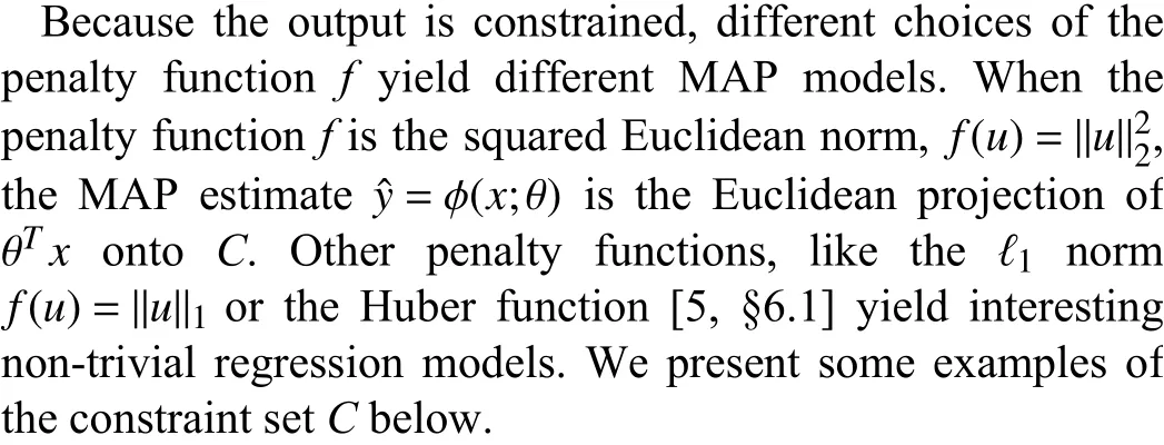
Nonnegative Regression:TakingC=Rm+(the set of nonnegativem-vectors) yields a MAP model for nonnegative regression, i.e., the MAP estimates in this model are guaranteed to be nonnegative.

Monotonic Output Regression:WhenCis the monotone cone, i.e., the set of ordered vectors cone,andevaluatingitrequiressolvinga convexquadratic program(QP);in this specialcase,once θTxhasbeen computed (which takesO(mn) time), evaluating the convex optimization model is equivalent to monotonic or isotonic regression [51], which takesO(m) time [52], meaning it has the same complexity as the standard linear regression model.

We note the distinction between traditional isotonic regression [51] and a convex optimization model with monotone constraint. In isotonic regression, we seek a single vector with nondecreasing components. In a convex optimization model with a monotone constraint, we seek a model that mapsx∈X to a predictionyˆ that always has nondecreasing components.

B. Classification

In (probabilistic) classification tasks, the outputs are vectors in the probability simplex, i.e.,

The outputycan be interpreted as a probability distribution over { 1,...,m} associated with an inputx∈X=Rn. The MAP estimateyˆ=φ(x;θ) is therefore the most likely distribution associated withx, under a particular densityp(y|x;θ). This includes as a special case the familiar setting in which each output is a label, e.g., a number in {1,...,m}, since the labelkcan be represented by a vectorysuch thatyk=1 andyi=0 fori≠k.

As a simple first example, consider the MAP model with density

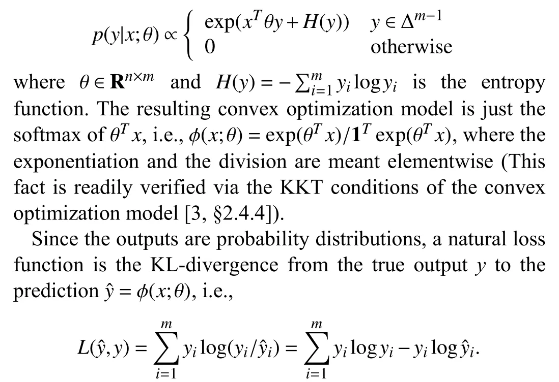
Discarding the constant termsyilogyi, which do not affect learning, recovers the commonly used cross-entropy loss [53,§2.6]. Using this loss function with the softmax model recovers multinomial logistic regression [53, §4.4]. This model can be made more interesting by simple extensions.

Constrained Logistic Regression:We can readily add constraints on the distributionyˆ. As a simple example, a boxconstrained logistic regression model has the form

whereCis a convex subset of Δm-1. There are many interesting constraints we can impose on the distributiony. As a simple example, the constraint set

where α ,β ∈Rmare vectors and the the inequalities are meant elementwise can be used to require thatyˆ have heavy tails, by making the leading and trailing components of α large, or thin tails, by making the leading and trailing components ofβ small. Another simple example is to specify the expected value of an arbitrary function on {1,...,m} underyˆ, which is a simple linear equality constraint onyˆ. More generally, any affine equality constraints and convex inequality constraints onyˆ may be imposed; these include constraints on the quantiles of the random variable associated withy, lower bounds on its variance, and inequality constraints on conditional probability distributions.

Piecewise-Constant Logistic Regression:A piecewiseconstant logistic regression model has the form

where the parameter is θ,

and λ ＞0 is a (hyper-) parameter. To the standard energy we add a total variation term that encouragesyto have few“jumps”, i.e., few indicesisuch thatyi≠yi+1,i=1,...,m-1[54, §7.4]. The larger the hyper-parameter λ is, the fewer jumps it will have.

C. Graphical Models

A Markov random field (MRF) is an undirected graphical model that describes the joint distribution of a set of random variables, which are represented by the nodes in the graph. An MRF associates parametrized potential functions to cliques of nodes, and the joint distribution it describes is proportional to the product of these potential functions. MRFs are commonly used for structured prediction, but learning their parameters is in general difficult [49, §8.3]. When the potential functions are log-concave, however, we can fit the parameters using the methods described in this paper.

is a convex optimization model. In this case, given a dataset of input-output pairs (x,y) , we can fit the parameter θ without evaluating or differentiating through the partition function.

MRFs with a similar clique structure have been proposed for various signal and image denoising tasks. We give a numerical example of fitting a quadratic MAP model of an MRF in Section VI.

We emphasize that the dependence onxcan be arbitrary;e.g., if the energy function were

wherefwere a neural network, the MAP model would remain convex.

IV. UTILITY MAXIMIZATION MODELS

We now consider the case where the outputyis a decision,and the inputxis a context or feature vector that affects the decision. We assume that the decisionyis chosen to maximize some given parametrized utility function

whereU(x,y;θ) is the utility of choosing a decisionygiven the contextxand the parameters θ, and is concave iny(Infinite values ofUare used to constrain the decisiony). The energy function in a utility maximization model is simply the negative utility

The resulting convex optimization model φ(x;θ) gives a maximum utility decision in the contextx. The same losses used for regression (see Section III-A) and classification (see Section III-B) can be used for utility maximization. The contextxmight include, for example, a total budget on the decisiony, prices that affect the decision, or availabilities that affect the decision.

whereU(y;θ) is some parametrized concave utility function,describing the utility of an allocation. In this simple case,φ(x;θ)gives the maximum utility allocation that satisfies the budget constraint.

The inputxis not limited to just the budget; it can also contain additional context that affects or constrain the decision. One important case is when the resource to be allocated is dollars, andxcontains the prices of the resource for each of the agents, denotedp∈Rm++. When there are prices, an allocation ofyidollars providesyi/piunits of some good to agenti. The utility in this case has form

where the division is meant elementwise, andU(z;θ) gives the utility of the agents receivingziunits of the resource,i=1,...,m. The resulting convex optimization modelφ(x;θ)gives the maximum utility allocation that satisfies the budget constraints, given the current prices.

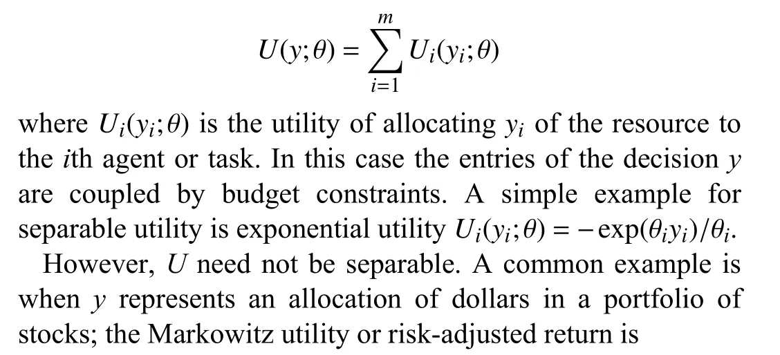
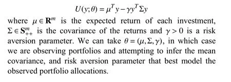
Utility Functions:A simple family of utility functions are the separable functions

V. STOCHASTIC CONTROL AGENT MODELS

In this section, we consider a setting in whichx∈X=Rnis the context or state of a dynamical system, andy∈Y=Rmrepresents the actions taken in that state. Our goal is to model the policy, i.e., the mapping from state to action, that the agent is using. In this section, we describe generic ways to model an agent’s policy with a convex optimization model. The convex optimization models we present are all instances of convex optimization policies commonly used for stochastic control[29]. When learning these models, one can use the same losses proposed for regression (see Section III-A).

In general, given a dataset describing an agent’s actions, we have no reason to believe that the agent chooses actions by solving a stochastic control problem. Nonetheless, choosing a model that corresponds to a policy for stochastic control can work well in practice. As we will see, our models involve learning the parameters in three functions that can be interpreted as dynamics, stage costs, and an approximate value function.

Approximate Dynamic Programming (ADP):One possible model of agent behavior is the ADP model [55, §6], which has the form

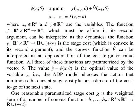
VI. NUMERICAL EXPERIMENTS

In this section we present four numerical experiments that mirror the examples from Sections III–V. The code for all of these examples can be found online1redacted.

Fig. 1. Monotonic output regression: linear regression (LR), convex optimization model (COM), true model (true). Left: validation loss. Right: predictions for a held-out input.

Fig. 2. Signal denoising. Predictions for a held-out input; least squares (LS), convex optimization model (COM), and true output (true).

We compare the convex optimization model to linear regression, using the standard sum of squares loss and no regularizer. The results for both of these methods are displayed in Fig. 1. On the left, we show the validation loss versus training iteration. The final validation loss for linear regression is 3.375, for the convex optimization model is 0.562, and for the true model is 0.264. We also calculated the validation loss of a convex optimization model with the linear regression parameters; this resulted in a validation loss of 1.511. While better than 3.375, this shows that here our learning method is superior to learning the parameters using linear regression and then projecting the outputs onto the monotone cone. On the right, we show both model’s predictions for a validation input.

Signal Denoising:Here, we fit the parameters in a quadratic MRF (see Section III-C) for a signal denoising problem. We consider a denoising problem in which each inputx∈Rnis a noise-corrupted observation of an outputy∈Rm, wheren=m.The goal is to reconstruct the original signaly, given the noise-corrupted observation. We model the conditional density ofygivenxas

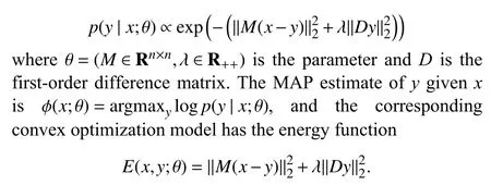
The first term says thatxshould be close toy, as measured by the squared quadraticM-norm, while the second term says that the entries ofyshould vary smoothly. WhenM=I, this model is equivalent to least-squares denoising with Laplacian regularization. We note that this convex optimization model has the analytical solution

We usen=100,m=100, andN=500 training pairs. Each outputyis generated by sampling a different scale factorafrom a uniform distribution over the interval [1,3], and then evaluating the cosine function at 100 linearly spaced points in the interval [0,2πa]. The outputs are corrupted by Gaussian noise to produce the inputs. We generate a covariance matrix Σaccording to

and then generate the components of each inputx

We generate 100 validation points in the same way. As a baseline, we use least-squares denoising with Laplacian regularization, sweeping λ to find the value which minimizes the error on the training set. The least-squares reconstruction achieves a validation loss of 0.090; after learning, the convex optimization model achieves a validation loss of 0.014. Fig. 2 compares a prediction of the convex optimization model with least squares and the true output, for a held-out input-output pair.

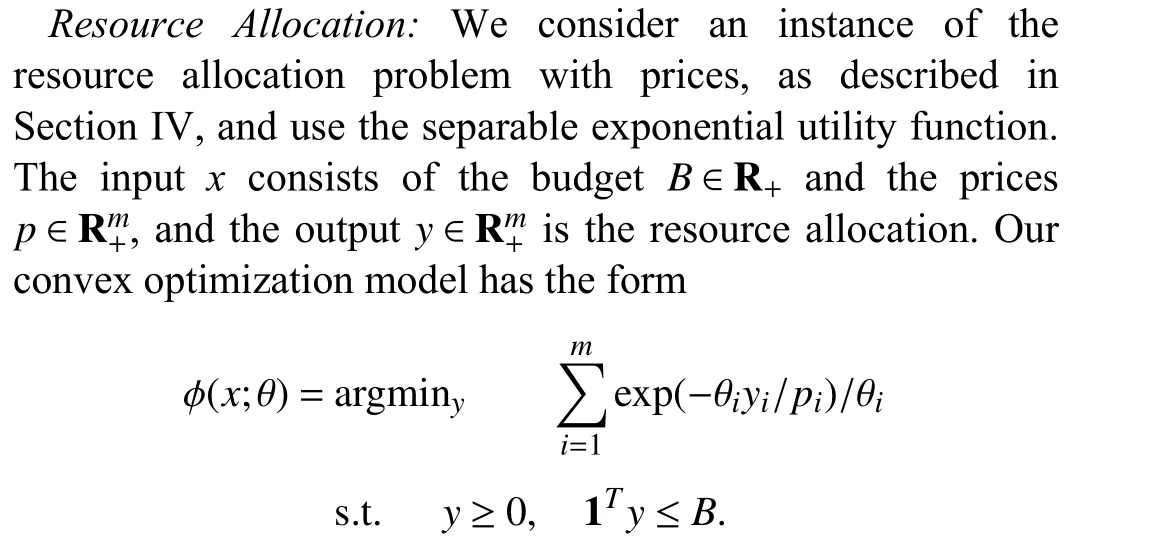
Fig. 3. Resource allocation. Left: validation loss versus iteration for logistic regression and our convex optimization model. Right: learned and true parameters.

Fig. 4. Constrained MPC. Left: validation loss for a neural network (NN), convex optimization model (COM), and true model (true). Right: learned and true parameters.

where ° denotes elementwise multiplication. In other words,we evaluate the true convex optimization model, multiply each output by a random number between 0.5 and 1.5, and rescale the allocation so it sums to the budgetB. We compare the convex optimization to logistic regression using the prices as features and the (normalized) allocation as the output. In Fig. 3 we show results for these two methods. On the left, we show the validation loss versus iteration for the convex optimization model, with horizontal lines for the validation loss of the logistic regression baseline and the true model. On the right, we show the learned and true utility function parameters, and observe that the learned parameters are quite close to the true parameters.

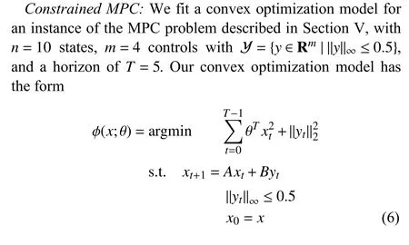
We use the mean-squared loss for the loss functionL, and train for 20 iterations. As a baseline, we compare against a two-layer feedforward ReLU network with hidden layer dimensionn, and with output clamped to have absolute value no greater than 0.5. The results are displayed in Fig. 4. The ReLU network achieves a validation loss of 0.071. The trained convex optimization model achieves a validation loss of 0.066, which is close to the validation loss of the underlying model. Additionally, the convex optimization model nearly recovers the true weights.