Novel Kriging-Based Decomposed-Coordinated Approach for Estimating the Clearance Reliability of Assembled Structures

Da Teng,Yunwen Feng,⋆,Cheng Lu,,Chengwei Fei,Jiaqi Liu and Xiaofeng Xue,⋆

1School of Aeronautics,Northwestern Polytechnical University,Xi’an,710072,China

2Department of Aeronautics and Astronautics,Fudan University,Shanghai,200433,China

ABSTRACT Turbine blisks are assembled using blades,disks and casings.They can endure complex loads at a high temperature,high pressure and high speed.The safe operation of assembled structures depends on the reliability of each component.Monte Carlo(MC)simulation is commonly used toanalyze structural reliability,but this method needs to run thousands of computations.In order to assess the clearance reliability of assembled structures in an efficient and precise manner,the novel Kriging-based decomposed-coordinated (DC)(DCNK)approach is proposed by integrating the DC strategy,the Kriging model and the importance sampling-based Markov chain(MCIS)technique.In this method,the DC strategy is used to decompose a multi-objective problem into many single-objective problems.The relationships between these many single-objectives and the overall objective are then coordinated.The Kriging model is applied to establish the limit state functions of the single-objectives and multi-objective problems, while the MCIS method is used to assess the structural assembled clearance reliability.Moreover, a highly nonlinear complex compound function is first utilized to verify the DCNK model from a mathematical perspective.Then,the reliability of an aeroengine high-pressure turbine(HPT)blade-tip radial running clearance(BTRRC)is analyzed to validate the DCNK approach by considering thermo-structural interaction.The analytical results show that the reliability is 0.9976 when the allowance value of the BTTRC is 1.7650×10−3 m.Compared with different methodologies(including direct simulation,the classical Kriging model,and the weighted response surface method(WRSM)),the proposed method holds obvious advantages in computing time and precision,as well as simulation efficiency and precision.The efforts of this paper provide a useful approach to analyzing assembled clearance reliability and contribute to the development of structural reliability theory.

KEYWORDS Kriging-based decomposed-coordinated approach; assembled clearance; reliability assessment; importance sampling; Markov chain

1 Introduction

Assembled structures usually involve many components in accordance with specific principles.These structures typically suffer from interaction loads between multi-physical fields.For instance,an aeroengine high-pressure turbine is assembled by blisks and casings, which enables it to endure thermal loads and structural loads during operation.Moreover, the overall safety of assembled structures is determined by the reliability of its components.As for assembled structures, if a component is not sufficiently reliable, the function of the entire system is affected, and a catastrophic accident can occur.Therefore, the clearance reliability of assembled structures must be analyzed by considering the randomness of influencing factors.

A number of direct methods have been proposed to analyze structural reliability.Rezaei et al.[1] applied Monte Carlo (MC)simulation with statistical learning theory to analyze the structural reliability of line systems.Zhang et al.[2] discussed the application of MC simulation for the purpose of analyzing the reliability of crankshafts.MC simulation is commonly applied to analyzing structural reliability in engineering and is usually regarded as the reference for validating analytical precision.Although MC simulation is highly precise when used for structural reliability assessment, it needs to run numerous simulations.In addition, the computational burden with MC simulation is obviously heavy.As a result, it is hard to analyze the reliability of assembled structures.Approximate analytic methods are simultaneously developed to address structural reliability estimation, e.g., first-order second-moment (FOSM), second-order second-moment (SOSM),and so forth.Liu et al.[3] employed the FOSM method to predict the reliability of chatter vibration in a milling system.Zhou et al.[4] presented a SOSM method for calculating the reliability index and failure probability of rock slopes.Shadab et al.[5] described a step-by-step algorithm to calculate the failure probability and safety index using an advanced FOSM (AFOSM)method.Zhang et al.[6] adopted the AFOSM approach to analyze the reliability of composite overwrapped cylinders.Lu et al.[7] studied an explicit second-order fourth-moment reliability index to assess the failure probability of simple and general parabolic approximations.Compared with MC simulation, the approximate analytic methods hold a certain analytical efficiency and are usually utilized to accomplish structural reliability evaluation based on the limit state function.However, these limit state functions are usually unknown for complex structures, and the scope of application for these techniques is limited in most cases.

In order to overcome the shortcomings of direct methods, indirect approaches (surrogate models)have been proposed to analyze the reliability of complex structures.Tandjiria et al.[8]studied the response surface method (RSM)for analyzing the reliability of laterally loaded piles.Kaymaz et al.[9] proposed the weighted response surface method for analyzing structural reliability.Gaspar et al.[10] analyzed the reliability of complex systems using the Kriging model.Gano et al.[11] developed a novel Kriging model-based updated strategy for optimizing variable fidelity.Jiang et al.[12] explored the support vector machine (SVM)in the reliability sensitivity analysis of mechanical structures.Xi et al.[13] evaluated the fault detection of an aircraft engine using the least squares SVM.Fei et al.[14] proposed an enhanced network learning model with an intelligent operator to evaluate the motion reliability of flexible mechanisms.Chang et al.[15]presented an artificial neural network with dynamic simulation and the FOSM method for analyzing the reliability of steering mechanisms.These efforts focus on single-objective reliability analysis without considering the effect of multi-objective correlation on structural reliability analysis.Some scholars investigated the multi-objective correlation reliability analyses of complex structures.Zhang et al.[16] proposed the multiple RSM and analyzed the reliability of turbine blisks with multi-failure modes.Fei et al.[17] evaluated probabilistic analyses in terms of their reliability and sensitivity for multi-component structures using the decomposition coordination strategy.However,the involved approaches still faced issues with analytical precision and computational efficiency,due to the use of the quadratic polynomial and thousands of simulations performed with the MC method.

In order to address the aforementioned issues, we develop a surrogate modeling strategy,namely the novel Kriging-based decomposed-coordinated (DCNK)approach, for the purpose of assessing structural assembled clearance reliability.In this case, the decomposed-coordinated (DC)strategy is used to decompose the multi-objective problem into many single-objective problems.Then, this strategy is used to coordinate the relationships between single-objectives and the overall objective.Furthermore, the Kriging model is applied to establish the limit state functions of the single-objective and multi-objective problems, while the importance sampling-based Markov chain(MCIS)technique is employed to assess structural assembled clearance reliability.In addition, we select a highly nonlinear compound function and an aeroengine high-pressure turbine (HPT)to validate the proposed method.

The rest of this paper is outlined as follows.In Section 2, the basic theory of structural assembled clearance reliability assessment with the DCNK approach is discussed.In Section 3, a highly nonlinear compound function is used to verify the DCNK approach in terms of predictive performance.In Section 4, the reliability analysis for the HPT blade-tip radial running clearance(BTRRC)is derived, so as to validate the analytical precision and computing efficiency of the DCNK method.Finally, in Section 5, the main conclusions are summarized.

2 Basic Theory

2.1 Assembled Clearance Reliability Assessment Process

In order to analyze the structural reliability of multiple objectives, the DCNK approach is developed by integrating the Kriging model, the DC strategy, the importance sampling principle and the Markov chain method.For the DCNK approach, the DC strategy is employed to decompose a “big” problem into many “small” problems, and to coordinate the “small” problems to process a “big”problem.Moreover, the Kriging model is used to derive the limit state functions of the related objectives, while the MCIS technique is adopted to generate samples and assess structural assembled clearance reliability.The structural assembled clearance reliability assessment process (including the DCNK approach)is shown in Fig.1.

As seen in Fig.1, there are four steps in assessing structural assembled clearance reliability with the DCNK approach.These are deterministic analysis, sample generation, DCNK modeling,and reliability assessment.The details are explained as below.

(1)Deterministic analysis—it is necessary to establish finite element (FE)models of objective structures, set constraints and boundary conditions, and execute the deterministic analysis based on the established FE models.

(2)Sample generation—it is necessary to determine the study time point depending on the variation in output response; ensure input parameters and their numerical features; obtain samples of input parameters using the Latin hypercube sampling (LHS)method [18]; calculate the output response with regard to the generated samples of input parameters; and subsequently obtain training and testing samples.

(3)DCNK modeling—it is necessary to establish the DCNK model based on the training samples and validate the established DCNK model using the testing samples.If the DCNK model prediction accuracy cannot satisfy the precision requirement, return to Step (2).Otherwise, move to Step (4).

(4)Reliability assessment—it is necessary to extract the candidate sampling pool using the MCIS method; obtain these values for the relevant output responses; and determine the structural assembled clearance reliability and output analysis results.

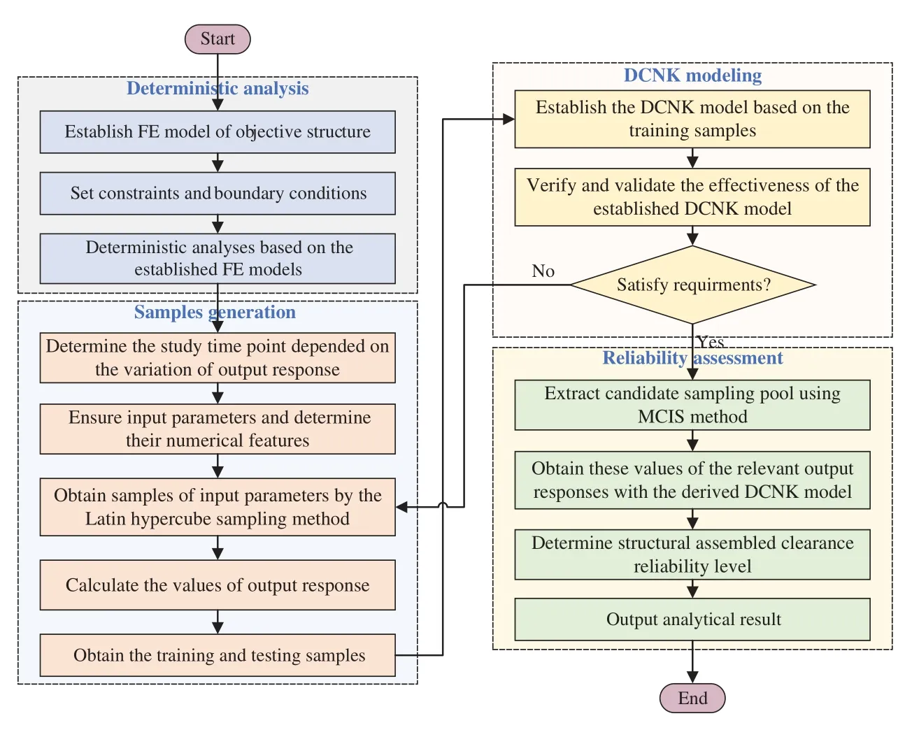
Figure 1: Structural multi-objective correlation reliability assessment process with the DCNK approach

2.2 Efficient Kriging-Based Decomposed-Coordinated Modeling

In this section, we elaborate on the basic theory underpinning the DCNK approach, including the Kriging model.

2.2.1 The Kriging Model

The Kriging model was first introduced into geostatistics by Krige [19], and is widely used in various subfields, such as reliability estimation, sensitivity analysis, and optimization design[20–22], due to its excellent fitting and predictive ability.In the Kriging model, the relationship between output responsey(x)andn-dimensional inputsx∈Rn[23] is denoted by:

wheref (x)=f1(x),f2(x),...,fp(x)is the basis functions of a regression model;pis the number of basis functions;β=expresses the regression coefficients of the basis functionsf(x); andZ(x)is a stationary Gaussian random process with an expected value of zero(i.e., E[Z(x)] = 0).The covariance is defined as:

whereR(·)is the correlation function between input variablesxiandxj(i,j= 1, 2,...,m)andmis the number of samples;δ2represents the variance;θis the Kriging model hyperparameter; and R is the the correlation parameter vector.The Gaussian correlation function is used as the form of the correlation function, i.e.,

whereldenotes the number of input variables;θk,andare thekth component ofθfor input samplesxiandxj, respectively.The optimal value of the hyperparameterθis approximated by the maximum likelihood function, i.e.,

whereRis the correlation matrix, which is expressed as:

whereYdenotes the vector of output responsesY=[y1,y2,...,ym]Tcorresponding to the input samples; andF=[f (x1),f (x2),...,f (xm)]T.The undetermined coefficientsβare obtained by:

The stochastic componentZ(x∗)at pointx∗is given by:

wherer(x∗)is the correlation vector between pointx∗and the sample points, i.e.,

2.2.2 Novel Kriging-Based Decomposed-Coordinated Strategy

Although the traditional Kriging model is suitable for general reliability problems, it is unable to effectively assess the clearance reliability of assembled structures, because this method requires multiple models to be established.In addition, the DC strategy proposed by Adomian has been utilized to approximate the complex compound function and performs well [24].Therefore, the DC strategy is introduced into the Kriging model to assess the clearance reliability of assembled structures.From a mathematical perspective, the DCNK approach can be executed as follows:(1)decompose the overall model for the assembled clearance into many sub-models for the substructures, (2)establish these sub-models in the form of the Kriging model, and (3)compile an overall model taking the relationship among the different objectives into account.In order to illustrate the details of the DCNK modeling, the four layers are treated as an example, as shown in Fig.2.These four layers are the overall model layer, the first sub-model layer, the second sub-model layer, and the variable layer.

As shown in Fig.2, the overall model layer presents the clearance function of the assembled structure; the first sub-model layer denotes the first subfunctions of the components; the second sub-model layer denotes the second subfunctions of the subcomponents; and the variable layer expresses the bottom parameters.The output response relationship between the overall model layer and the first sub-model layer is expressed byg(·);g(u)(·)denotes the output response relationship between theuth first sub-model layer andvth second sub-model layer; andg(uv)(·)represents the output response relationship between thevth second sub-model layer of theuth first sub-model layer and the variable layer.The DCNK modeling process is described as below.

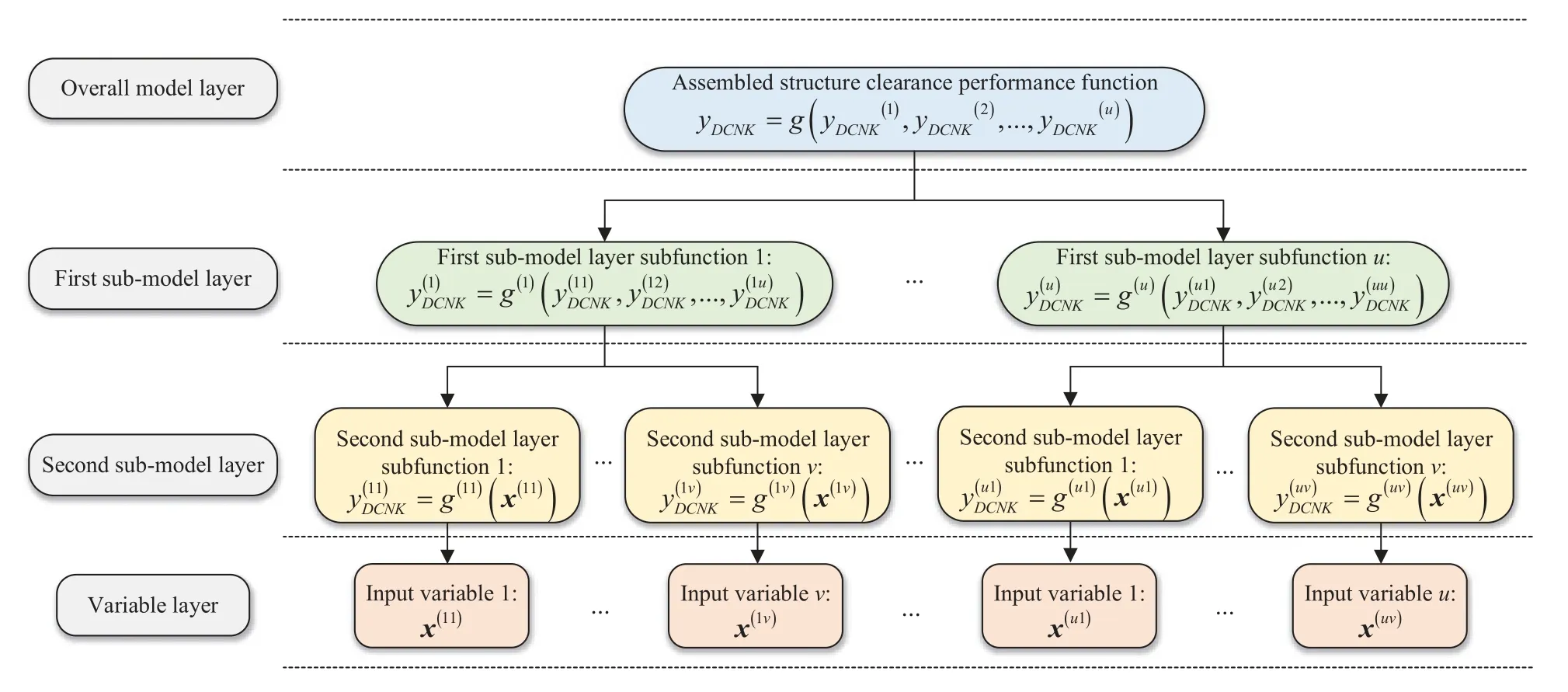
Figure 2: Decomposed and coordinated schematic diagram of the structural assembled clearance performance function

The assembled structure clearance function is given by:

Eq.(10)can be expressed as:

whereuis the number of output responses in the first sub-model layer; and(i= 1, 2,...,u)is the decomposed subfunctions of theith first sub-model layer.This is represented by:

wherevis the number of output responses in the second sub-model layer; and(j= 1,2,...,v)indicates the decomposed subfunctions of thejth second sub-model layer in theith first sub-model layer.This is represented by:

wherex(i j)is thejth decomposed subfunction in the second sub-model layer of theith first submodel layer.

Based on Eq.(1), thejth decomposed model in the second sub-model layer of theith first sub-model layer is denoted by:

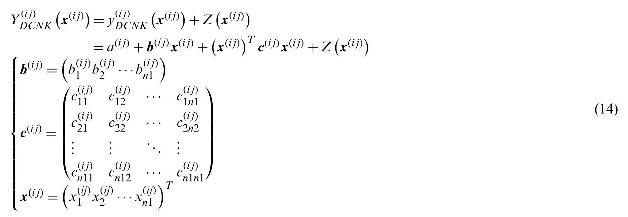
wherea(i j),b(i j), andc(i j)are the undetermined coefficients of the constant term, line term,and quadratic term, respectively; andn1represents the number of input variables in thejth decomposed model of the second sub-model layer of theith first sub-model layer.

According to the Kriging model, theith decomposed model in the first sub-model layer is given by:

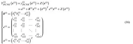
wherea(i j),b(i j), andc(i j)are the undetermined coefficients; andn2is the number of input variables in theith first sub-model layer.

Similarly,is treated as the input variables of the overall model layer, i.e.,

The overall model layer is derived in the form of the Kriging model, i.e.,

Eq.(18)is denoted by:

wherea,b, andcare the undetermined coefficients of the constant term, linear term, and quadratic term, respectively.

Furthermore, the limit state function of the assembled structure clearance is given by:

whereis the allowable value of the assembled structure clearance.

Through the above analysis, the limit state function of the assembled structure clearance is decomposed into many subfunctions.Each subfunction is established based on the Kriging model,and then the overall model of the assembled structure clearance function is derived based on the relationship between the whole object and its sub-objects.

2.3 Reliability Assessment with the MCIS

In this section, the probabilistic analysis is conducted with the limit state function of the assembled structure clearance.The candidate sample pool is determined via MCIS simulation.The prediction values of the limit state function are acquired using the DCNK model.

2.3.1 Importance Sampling-Based Markov Chain Simulation

The Markov chain based on the Metropolis-Hasting algorithm is adopted in order to simulate the conditional samples of the failure domain, and to improve their efficiency [25].Conditional samples are simulated in the failure domain using a Markov Chain [26] by following the steps outlined below:

(1)Define the stationary distribution of the Markov Chain.According to the analysis results,the failure probability of the assembled structure clearance is given by:

where the vectorxis uncertain input variables;f(x)indicates the joint probability density function(PDF);G(x)is the limit state function, whereG(x)> 0 indicates a safety state andG(x)<0 presents a failure state; andPfrepresents the failure probability of the reliability analysis problem.The limit distribution of the Markov Chain is defined as the joint PDFq(x|F)in the failure domainF, whenMconditional samples=1,2,...,M)in the failure domainFare simulated.Theq(x|F)is expressed as:

whereIF(x)is a failure indicator function.

(2)Select the proper proposal distribution.The proposal distributionf∗(ε|x)controls the transition from one state to another in the Markov Chain process.In this paper, then-dimensional uniform distribution with symmetry is selected as the proposal distribution.Thef∗(ε|x)is denoted by:

whereεiandxiare theith components of then-dimensional vectorsεandx, respectively;liis the length of the side in thexidirection of then-dimensional hyper-polyhedron centered onx.The choice ofligoverns the maximum allowable distance that the next sample can depart from the current one.In this study,litakes an empirical value ofwhereσxiis the variance of input variables.

(3)Select the initial state of the Markov Chain.The initial state of the Markov Chain should follow a limit distributionq(x|F)and can be determined by engineering.

(4)Determine thekth stateof the Markov Chain.Thekth states generated based on the (k−1)th stateand the proposal distribution.The alternative stateεis generated by the proposal distributionf∗(ε|x).The conditional PDF ratiorof the alternate state to the previous state is calculated in Eq.(24):

According to the Metropolis-Hasting algorithm,=εandare assumed with probability min(1,r), i.e.,

whererandom[0, 1] is a uniformly distributed random number in [0, 1].

(5)GenerateMconditional samples following a limit distributionq(x|F).The determinedkth stateof the Markov Chain is repeated.M states of the Markov Chain are generated as the conditional samples within the failure domain following a limit distributionq(x|F).

In summary, the conditional samples=1,2,...,M)in the failure domain are obtained with respect to a limit distributionq(x|F).Compared with the samples for the joint PDF values in the failure domain, the sample for the largest joint PDF value in the failure domain is obtained,which is used to approximate the most probable point (MPP)[27].The MPP obtained by the joint PDF is displayed in Fig.3.

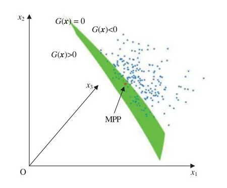
Figure 3: MPP obtained using the joint PDF

In Fig.3, the green face denotes the limit state surface, while the blue points represent the conditional samples in the failure domain generated by MC simulation.The red point is the MPP,whilex1,x2, andx3denote the components ofx.

The importance sampling PDF is introduced to solve the failure probability [28], i.e.,

whereh(x)is the importance sampling PDF; andRnis the real number space.

As the MPP is the point with the largest joint PDF value in the failure domain, the importance sampling PDF is constructed at the MPP, i.e., the optimal importance sampling PDFh(x)is computed by:

The MCIS can be used to simulate the failure domain samples without information concerning the true samples, such that it may determine the MPP with the largest joint PDF value and thus construct the importance sampling PDF.Therefore, the MCIS is suitable for the highly nonlinear and high-dimensional limit state function.

2.3.2 Reliability Analysis

In order to analyze the reliability of the assembled structure clearance efficiently, the MCIS and DCNK models are combined.The MCIS is used to construct the importance sampling PDFhopt(x)and the DCNK model is employed to generate the prediction values instead of the assembled clearance function values.

The flowchart for analyzing the assembled structure clearance reliability is summarized in Fig.3.The specific process is as follows [29,30].

(1)Construct the importance sampling PDFhopt(x)using the MCIS.

(2)Generate the candidate sampling poolSISusing thehopt(x).NISimportance sampling samples are generated as the candidate samplesSIS=｛x1,x2,...,xNIS｝.

(3)Compute the DCNK modelGk(xp)(p= 1, 2,...,NIS)based on the candidate training sample setsSISand use the DACE toolbox for Kriging [31], whereGk(xp)denotes the limit state function when the importance sampling samples arexp.The Gaussian is chosen in the correlation model and the regression model is constant.

(4)Calculate the failure probabilityPfusing the failure indicator function valuesIF(xp)judged by the DCNK modelGk(xp).

3 Numerical Example

In order to validate the proposed DCNK model by comparing the Kriging model and the WRSM, a highly nonlinear complex compound function is considered as the case study.All computations are completed on a 64-bit desk computer with Intel Core i5–10400 of 2.9 GHz CPU and 32 GB RAM.

3.1 Compound Function Approximation

In the numerical example,y(x)denotes the complex compound function, while the subfunctions are represented byy(1)(x),y(2)(x), andy(3)(x).x= [x1,x2,...,x6] denotes the input variables,which are assumed to be mutually independent and normally distributed as shown in Tab.1.

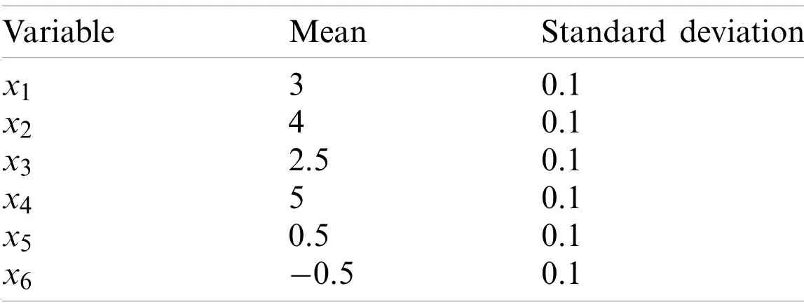
Table 1: Distribution parameters of the input variables

The output response relationship between the complex compound function and subfunctions is expressed byg(·), i.e.,

In order to establish the DCNK model, 50 samples are obtained using the LHS method in accordance with the input variables’distribution parameters.30 samples are used as training samples to establish the DCNK model, while the remaining 20 samples are taken as the testing samples to verify the performance of the DCNK model.The decomposed and coordinated models of the subfunctions are given by:

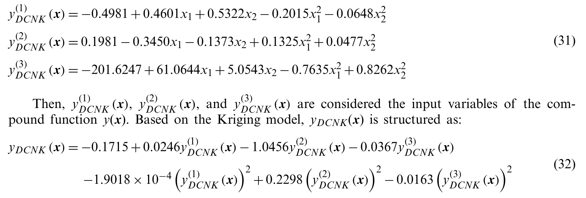
Using these 30 samples as the training samples, a Kriging modelykriging(x)for the complex compound functiony(x)can be constructed as:

Similarly, the WRSM modelyWRSM(x)for the complex compound functiony(x)is given by:

3.2 Verifying the DCNK Model’s Accuracy

The accuracy of the DCNK model is tested using the remaining 20 samples.Using the true response for the compound function as a reference, the prediction error of the DCNK model is calculated by comparing the Kriging model and the WRSM.The prediction errors, including the absolute error (Ea)and the average absolute error (Eav), are computed by:

wherey∗(xi)(i= 1, 2,...,m)is theith prediction response for the surrogate model to theith test samples; andytrue(xi)denotes the true response for the complex compound function against theith testing samples.

The input variablex(x1,x2,x3,x4,x5,x6)is shown in Tab.2.The results of the prediction analysis from the DCNK model based on the testing samples are shown in Tabs.3 and 4, and Fig.4.

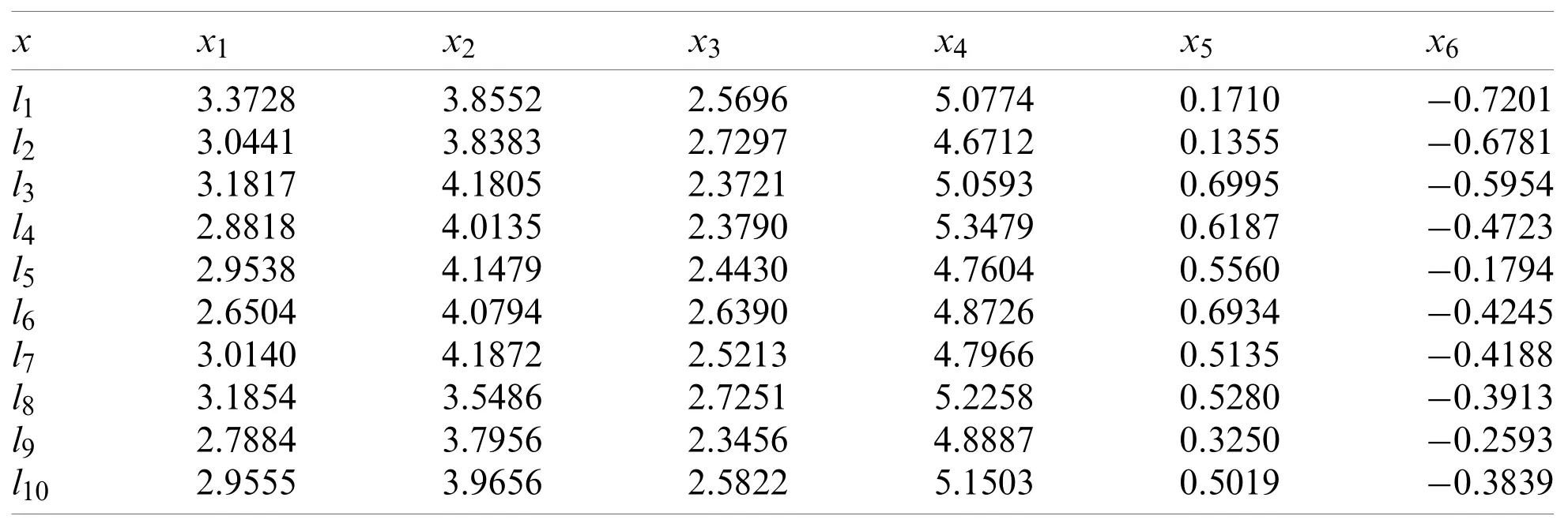
Table 2: The input response for the test samples

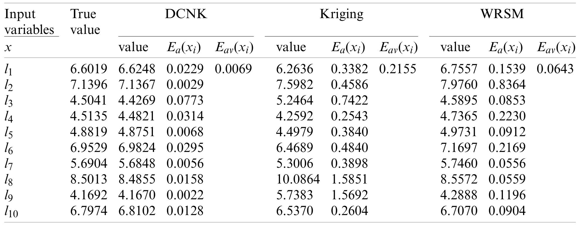
Table 3: The output response and errors for the test samples

As seen in Tab.3, the average absolute error of the DCNK model is only 0.0069, which is far below those of the Kriging model and the WRSM (i.e., 0.2155 and 0.0643).The prediction accuracy of the DCNK model is 99.3%,which is closer to the true value than those of the Kriging model and the WRSM.As shown in Tab.4, the modeling and prediction time of the DCNK model are smaller than those of the Kriging model and the WRSM.The reason for this is that the complex compound function is decomposed into the subfunctions using the DC strategy, with the parallel calculation of subfunctions saving substantial time in the modeling and prediction stages.

Table 4: Modeling and prediction times for the DCNK model, the Kriging model and the WRSM

For different test samples, the absolute error curves of the DCNK model, the Kriging model and the WRSM are shown in Fig.4.As illustrated in Fig.4, the absolute error curve of the DCNK model is smaller than those in the Kriging model and the WRSM.

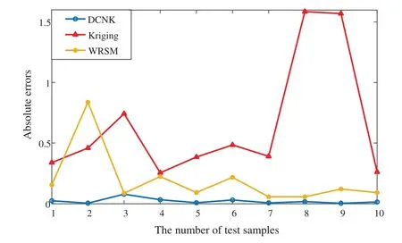
Figure 4: The absolute error curves for the DCNK model, the Kriging model and the WRSM

In summary, the DCNK model performs better with regard to the complex compound function with large-scale parameters for a highly nonlinear problem.It is indicated that the DCNK model is more robust and stable as a model.Therefore, the DCNK method is used to estimate the assembled clearance reliability of an aeroengine HTP BTRRC.

4 Modeling and Simulation of the HTP BTRRC

The BTRRC refers to a critical assembly relationship in an aeroengine high-pressure turbine.Its running clearance seriously affects the performance and reliability of an aeroengine.In this section, we consider the BTRRC of an aeroengine as the study object for the purpose of verifying the proposed DCNK approach.

4.1 HTP BTRRC Deterministic Analysis

Aeroengine turbines endure complex loads during operation, such as thermal loads, and structural loads.In order to analyze the thermo-structural coupling, we simplify the HPT model by ignoring tenons, pin holes, and cooling holes [32,33].The climb phase of an aeroengine is selected as the study object [34].The HPT BTRRC analysis is divided into the radial deformation analysis of the blisks and casings.The FE models are shown in Fig.5.

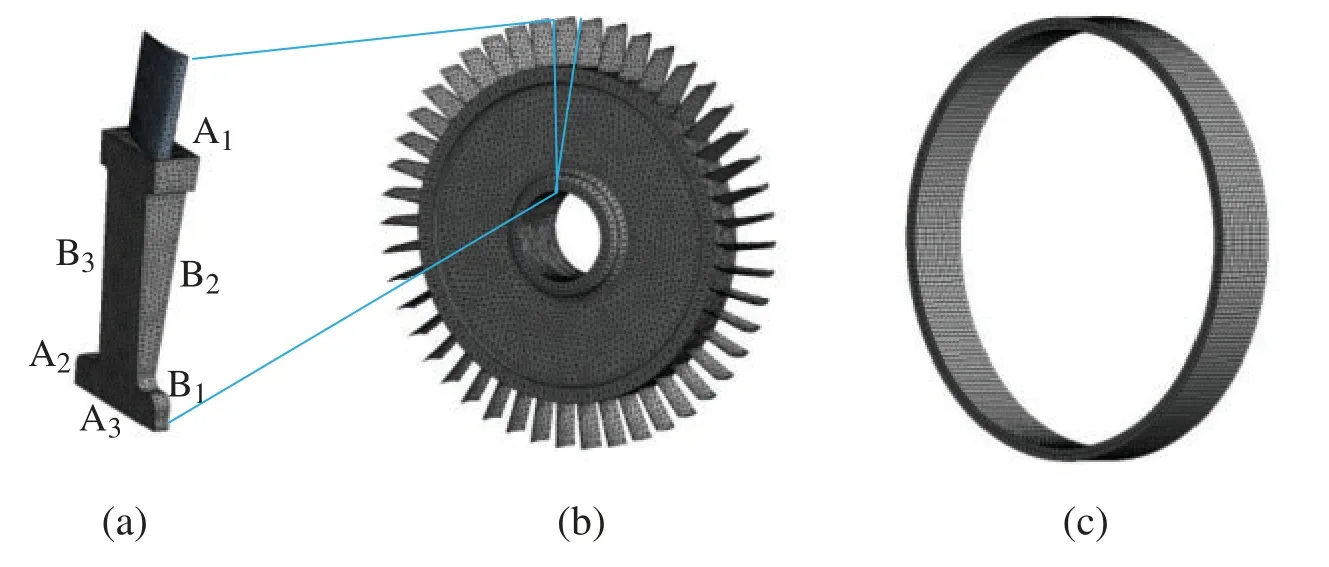
Figure 5: FE models of the turbine blisks and casings (a)1/46 turbine blisk (b)Whole turbine blisk (c)Turbine casing

The radial deformations of the blisks and casings are the largest in the climb phase of aeroengines [35], as shown in Fig.6.

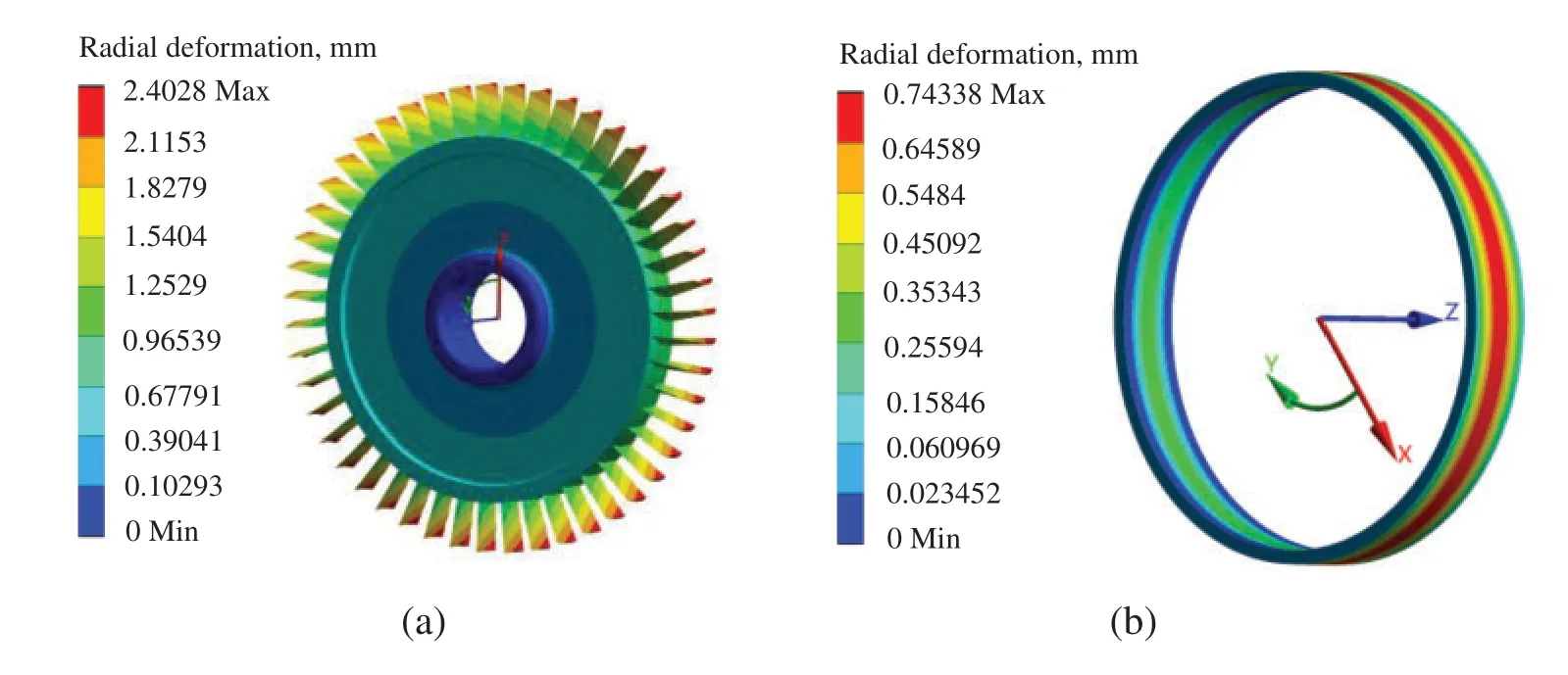
Figure 6: Distributions of radial deformations of the blisks and casing (a)Blisk (b)Casing

4.2 DCNK Modeling of the HTP BTRRC

The key parameters are selected as random variables in BTRRC analysis [36–38].The random variables shown in Tab.5 are assumed to be mutually independent and normally distributed.In Tab.5,ωis the rotor speed,ρis the material density,Tis the temperature, andαis the surface coefficient of heat transfer.For the blisk variables, the subscripts d1, d2, and d3 ofαrepresent the areas of B1, B2, and B3, respectively, while the subscripts b1, b2, and b3 ofTandαdenote the blade at the blade-tip, upper section, and lower section, respectively.For the casing variables, the inside and outside temperatures of the casing are represented byTiandTo.The casing interior is divided into four regions A, B, C, and D, which are indicated by the subscripts c1, c2, c3, and c4 ofα, respectively.The subscript o ofαdenotes the casing exterior.

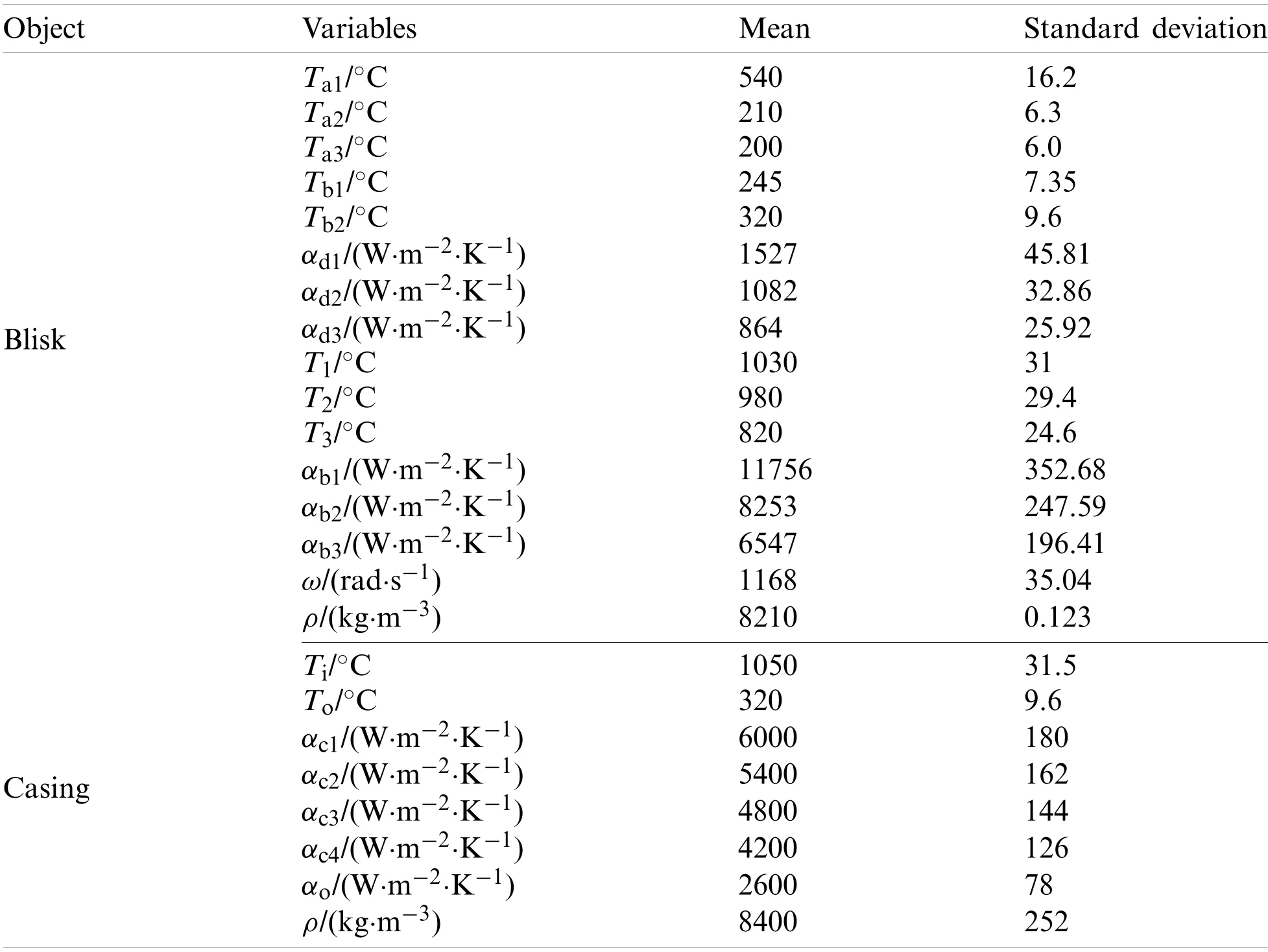
Table 5: The distributions of the random variables

Based on the characteristics of the random variables in Tab.5, we extracted 282 samples of random variables using the LHS method.These outputs, which correspond to the related input samples, are obtained via multiple deterministic analyses.These samples are used to establish the DCNK models for the radial deformationsYbandYcof the blisks and casings, i.e.,

The BTRRC coordinated modelYBTis obtained byYcandYb, such that:

The limit state function of the BTRRC is denoted as:

whereYallowis the allowance value of the BTTRC, which is usually determined by 3 sigma levels.

4.3 Assessing the HTP BTRRC’s Reliability

The convergence analysis of the BTRRC limit state function is performed using different DCNK approach simulations.The results of the convergence analysis are shown in Fig.7.

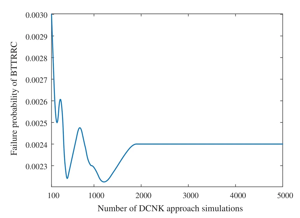
Figure 7: Convergence analysis with different DCNK approach simulations

As shown in Fig.7, the BTRRC deformations fluctuate when the number of DCNK approach simulations is less than 2 × 103.Moreover, the BTRRC deformation gradually converges to 0.0024.

The simulation history and BTRRC deformation distribution histogram are shown in Fig.8.

As demonstrated in Fig.8, the BTRRC deformation is normally distributed with a mean of 1.7635 × 10−3m and a standard variance of 2.1420 × 10−3m.The allowance valueYallowof the BTTRC is 1.7650 × 10−3m which is determined by the 3-sigma principle.Therefore, the failure probability is 0.0024 and the reliability is 0.9976.

4.4 Simulation Performance Verification

In order to verify the DCNK approach in the BTRRC reliability assessment, the BTRRC limit state equation is simulated for different times using the four methods (MC simulations, the Kriging model, the WRSM, and the DCNK model).The failure probabilities and reliability are listed in Tab.6.

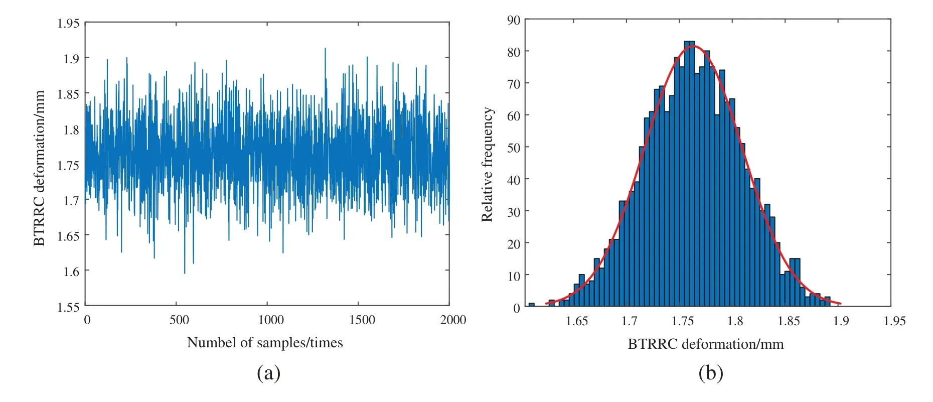
Figure 8: Simulation history and BTRRC deformation distribution (a)Simulation history of the BTRRC deformation (b)Distribution of the BTRRC deformation

Table 6: The results of the BTRRC probabilistic analysis under the four methods

As illustrated in Tab.6, the failure probability and reliability of the DCNK approach converge to constants when the number of simulations is 2000.The simulations under the DCNK approach are far less than under the WRSM and the Kriging model.The precision of the DCNK approach(99.98%)is higher than those of the Kriging model and the WRSM (i.e., 99.92% and 99.94%,respectively)in the BTRRC reliability assessment.Therefore, the DCNK approach can produce better simulations for the purpose of the HTP BTRRC analysis, compared to the Kriging model and the WRSM.

5 Citations

In this paper, a new surrogate model method is proposed for the probabilistic analysis involving assembled structure clearance with high nonlinearity and hyperparameters.In order to establish the relationship between the input parameters and output response of the assembled clearance, the DCNK approach is proposed by combining the Kriging model and the DC strategy.The MCIS method and the DCNK model are used to assess the reliability of the assembled structure clearance.The effectiveness and applicability of the DCNK approach are verified numerically and by assessing aeroengine HTP BTRRC reliability.Some conclusions are summarized as follows:

(1)The average absolute error of the DCNK model is 0.0069, which is far less than that of the Kriging model and the WRSM (i.e., 0.2155 and 0.0643, respectively).

(2)The prediction accuracy of the DCNK model is 99.3%, which is closer to the true value than that of the Kriging model and the WRSM (78.5% and 93.6%, respectively).

(3)The modeling and prediction time for the DCNK model (0.0829 s)are smaller than those of the Kriging model (0.1077 s)and the WRSM (15.2695 s).

(4)The failure probability is 0.0024 and reliability is 0.9976 when the allowance value of the BTTRC is 1.7650 × 10−3m.The failure probability and reliability of the DCNK approach converges when the number of samples reaches 2000.

(5)The precision of the DCNK approach (99.98%)is higher than that of the Kriging model and the WRSM (99.92% and 99.94%).

In summary, compared to the Kriging model and the WRSM, the DCNK approach performs better for the complex compound function with large-scale parameters for a highly nonlinear problem, when modeling approximation accuracy (modeling accuracy)and simulation performance(computational efficiency and precision).The present study offers an effective approach to highly nonlinear assembled structures, and promising insights for the probabilistic optimal design of the HPT BTRRC.

Funding Statement:This paper is supported by the National Natural Science Foundation of China(51875465)and the Civil Aircraft Scientific Research Project.The authors would like to thank their generous supports.

Conflicts of Interest:The authors declare that they have no conflicts of interest to report regarding the present study.