A New Method to Evaluate Linear Programming Problem in Bipolar Single-Valued Neutrosophic Environment

Jamil Ahmed,Majed G.Alharbi,Muhammad Akramand Shahida Bashir

1Department of Mathematics,University of Gujrat,Gujrat,Pakistan

2Department of Mathematics,College of Arts and Sciences,Methnab,Qassim University,Buraydah,Saudi Arabia

3Department of Mathematics,University of the Punjab,New Campus,Lahore,Pakistan

ABSTRACT A bipolar single-valued neutrosophic set can deal with the hesitation relevant to the information of any decision making problem in real life scenarios,where bipolar fuzzy sets may fail to handle those hesitation problems.In this study, we first develop a new method for solving linear programming problems based on bipolar singlevalued neutrosophic sets.Further, we apply the score function to transform bipolar single-valued neutrosophic problems intocrisp linear programming problems.Moreover,we apply the proposed technique tosolve fully bipolar single-valued neutrosophic linear programming problems with non-negative triangular bipolar single-valued neutrosophic numbers (TBSvNNs)and non-negative trapezoidal bipolar single-valued neutrosophic numbers(TrBSvNNs).

KEYWORDS Bipolar single-valued neutrosophic numbers; score function; trapezoidal numbers; linear programming

1 Introduction

The origin of linear programming is the 1940s (World War II).Linear programming (LP)has a linear objective function and a group of linear equalities and inequalities.LP was first used in petroleum manufacturing.Well elaborated data with much information is used for LP problems.On the other hand in real life problems the accuracy of data is often deceitful and affects the optimal solution of LP problems.Probability distribution cannot transact with inaccurate and unclear information.

In 1965, Zadeh [1] introduced fuzzy sets to handle imprecise information.Atanassove [2]gave the concept of intuitionistic fuzzy sets.The intuitionistic fuzzy sets consider both truthmembership and falsity-membership.Intuitionistic fuzzy sets can only handle incomplete information and not the indeterminate information and inconsistent information which exist commonly in the belief system.In 1998, Smarandache [3] presented the notion of neutrosophic set theory.Smarandache [3] and Wang et al.[4] defined a single-valued neutrosophic set which takes the value from the subset of [0, 1].Deli et al.[5] introduced the concept of bipolar single-valued neutrosophic sets as an extension of bipolar fuzzy sets [6].

Bellman et al.[7] first introduced the concept of decision making in a fuzzy environment.Zimmermann [8] proposed the fuzzy programming technique to solve the multiobjective linear programming problem under a fuzzy environment.Tanaka et al.[9] studied fuzzy-mathematical programming.Lotfi et al.[10] discussed full fuzzy linear programming (FFLP)problems in which all parameters and variables are triangular fuzzy numbers.They used the concept of the symmetric triangular fuzzy number and introduced an approach to defuzzify a general fuzzy quantity.Allahviranloo et al.[11] suggested a method to solve FFLP problems by using a ranking function.Veeramani et al.[12] suggested a method to deal with a kind of fuzzy linear programming (FLP)problem involving symmetric trapezoidal fuzzy numbers.Kumar et al.[13–15] worked on fuzzy linear programming by using non-negative and unrestricted variables to find optimal solutions of FFLP problems.By using trapezoidal fuzzy numbers Behera et al.[16,17] presented a new method to solve linear programming (LP)problems.Najafi et al.[18,19] proposed an efficient technique for solving FFLP by using unrestricted parameters and variables.Moloudzadeh et al.[20] suggested a simple method to solve an arbitrary fully fuzzy linear system.Akram et al.[21] proposed a method to solve LR-bipolar fuzzy linear systems.Mehmood et al.[22] suggested a method to solve fully bipolar fuzzy linear programming (FBFLP)problems by using non-negative bipolar fuzzy numbers and unrestricted bipolar fuzzy numbers with equality constraints.They transformed FBFLP problem into a crisp linear programming problem and achieved the exact bipolar fuzzy optimal solution.

Intuitionistic optimization is an extension of fuzzy optimization.Garg et al.[23] used an Intuitionistic fuzzy optimization method for solving reliability optimization problems in interval environment.Angelov [24] worked in an intuitionistic fuzzy environment.Many researchers solved intuitionistic fuzzy linear programming (IFLP)problems by using triangular intuitionistic fuzzy numbers [25–29].In an interval-valued intuitionistic fuzzy environment, Bharati et al.[30] gave the solution of multiobjective linear programming problems.Parvathi et al.[31] proposed linear regression analysis in an intuitionistic fuzzy environment and also worked on intuitionistic fuzzy linear programming [32].

The first contribution of neutrosophic linear programming theory was studied by Abdel-Basset et al.[33].They introduced the neutrosophic linear programming (NLP)models in which the parameters are presented with trapezoidal neutrosophic numbers(TrNNs)and presented a technique for solving them.Das et al.[34] worked to solve NLP problems by using mixed constraints.Bera et al.[35] proposed the Big-M simplex technique to solve NLP problems.Edalatpanah [36]proposed a new direct algorithm for solving the LP problems including neutrosophic variables.Hussian et al.[37] proposed LP problems based on neutrosophic environment.Khalifa et al.[38]suggested a method to solve NLP by using single-valued neutrosophic numbers(SvNNs).Recently,Akram et al.[39,40] have presented new methods to solve Pythagorean fuzzy linear programming problems.

In this paper, we are going to extend the NLP problems into bipolar single-valued neutrosophic linear programming(BSvNLP)problems in which all the coefficients, variables and right hand side are represented by bipolar single-valued neutrosophic numbers(BSvNNs).The fully bipolar single-valued neutrosophic linear programming(FBSvNLP)problems are superior to crisp linear programming (CLP)problems and up to our knowledge, there is no work in literature onFBSvNLP.TheBSvNLPproblems are more appropriate to avert unrealistic modeling.This is unique research that deals with LP problems in aBSvNenvironment withTBSvNNsandTrBSvNNs.Score function is used to convertBSvNNsto CLP problems.

This paper has been categorized as follows: In Section 2, basic concepts ofBSvNs,TBSvNNs,TrBSvNNsand their arithmetic operations are discussed.In Section 3, methodology for solvingFBSvNLPproblems are explained.In Section 4, some examples and practical models are solved.In Section 5, comparative analysis is depicted and conclusion is given in Section 6.The list of acronyms used in the research paper is given below:

BSvNNBipolar single-valued neutrosophic number

TBSvNNTriangular Bipolar single-valued neutrosophic number

TrBSvNNTrapezoidal Bipolar single-valued neutrosophic number

LPP Linear programming Problem

FFLP Fully fuzzy linear programming

2 Preliminaries

Definition 2.1.[5] LetXbe a non-empty set.A bipolar single-valued Neutrosophic setinXis an object having the form

whereT+(x),I+(x),F+(x):X→[0,1] andT−(x),I−(x),F−(x):X→[−1,0].The positive membership degreeT+(x),I+(x),F+(x)denotes the truth membership, indeterminate membership and falsity membership of an elementx∈Xcorresponding to a bipolar neutrosophic set ˜Bsimilarly negative membership degreeT−(x),I−(x),F−(x)denotes the truth membership, indeterminate membership and falsity membership of an elementx∈Xto some implicit counter-property corresponding to a bipolar neutrosophic set

Definition 2.2.Based on [15], we define aTBSvNNdefined on R

is said to be non-negativeTBSvNNif and only ifai≥0 andei≥0.wherei=1,2,3 such thatai≤bi≤cisimilarlyei≤fi≤gialsoχp,βp,ζp∈[0,1] andαn,ϕn,νn∈[−1,0]⊂R.

Definition 2.3.Based on [15], we define aTrBSvNNdefined on R

is said to be non-negativeTrBSvNNif and only ifai≥0 andei≥0.wherei=1,2,3 andai≤bi≤ci≤disimilarlyei≤fi≤gi≤hialsoχp,βp,ζp∈[0,1] andαn,ϕn,νn∈[−1,0]⊂R.

Definition 2.4.[30] LetM=≺(T+(x),I+(x),F+(x),T−(x),I−(x),F−(x))≻be aBSvNNthen the score function is presented by:

Definition 2.5.Based on [41], we define aBSvNNon R is aBSvNset such that:

whereχp,βp,ζp∈[0,1] andαn,ϕn,νn∈[−1,0]⊂R whose true membership values are given as:

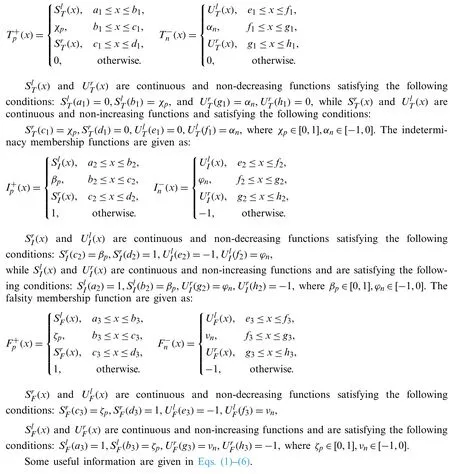
whose truth, indeterminacy and falsity membership functions are presented by:

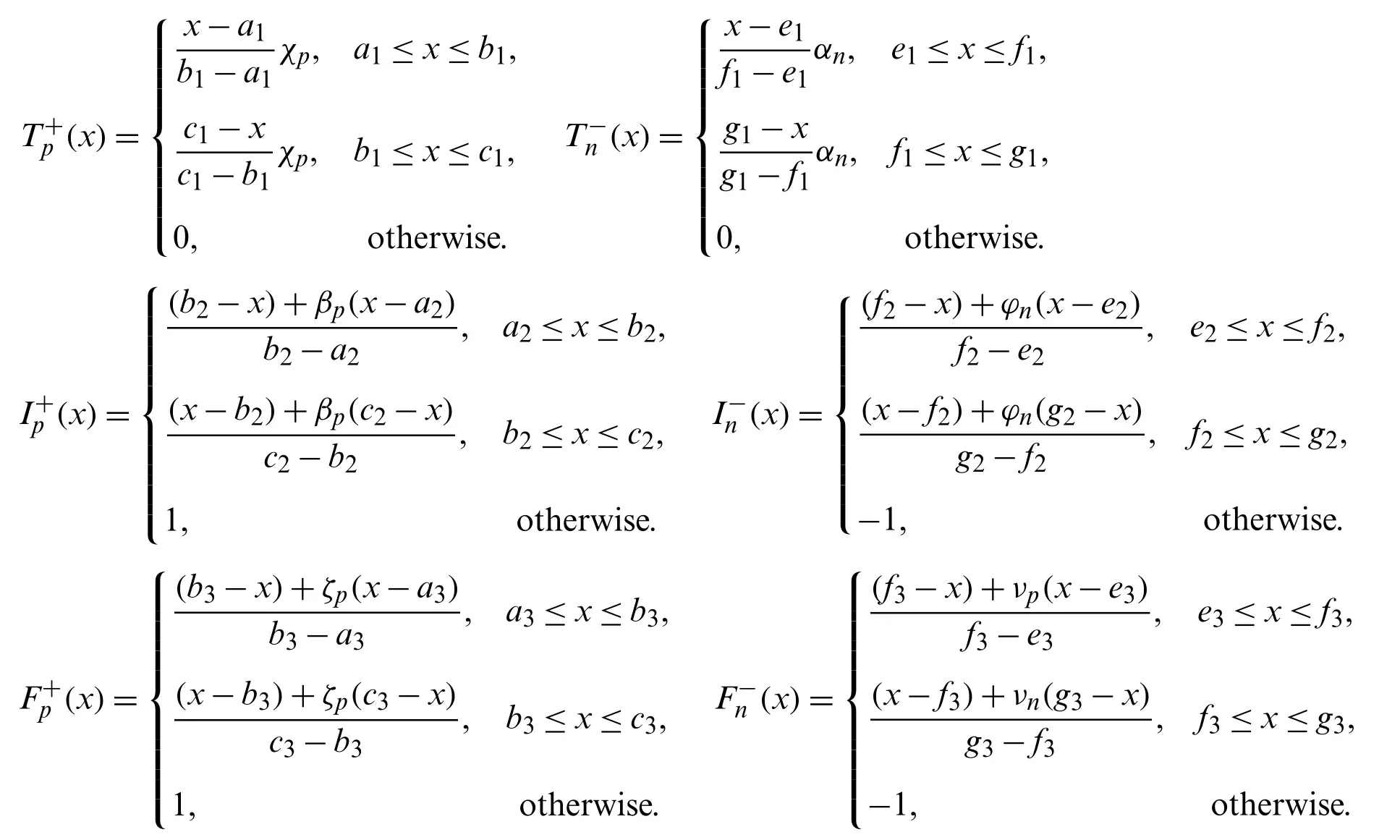
whereχp,βp,ζp∈[0,1] andαn,ϕn,νn∈[−1,0]⊂R.

Definition 2.8.Based on [42], we defineTrBSvNNdefined R denoted by:=≺([a1,b1,c1,d1];χp),([a2,b2,c2,d2];βp),([a3,b3,c3,d3];ζp),([e1,f1,g1,h1];αn),([e2,f2,g2,h2];ϕn),([e3,f3,g3,h3];νn)≻

whose truth, indeterminacy and falsity membership functions are presented by:

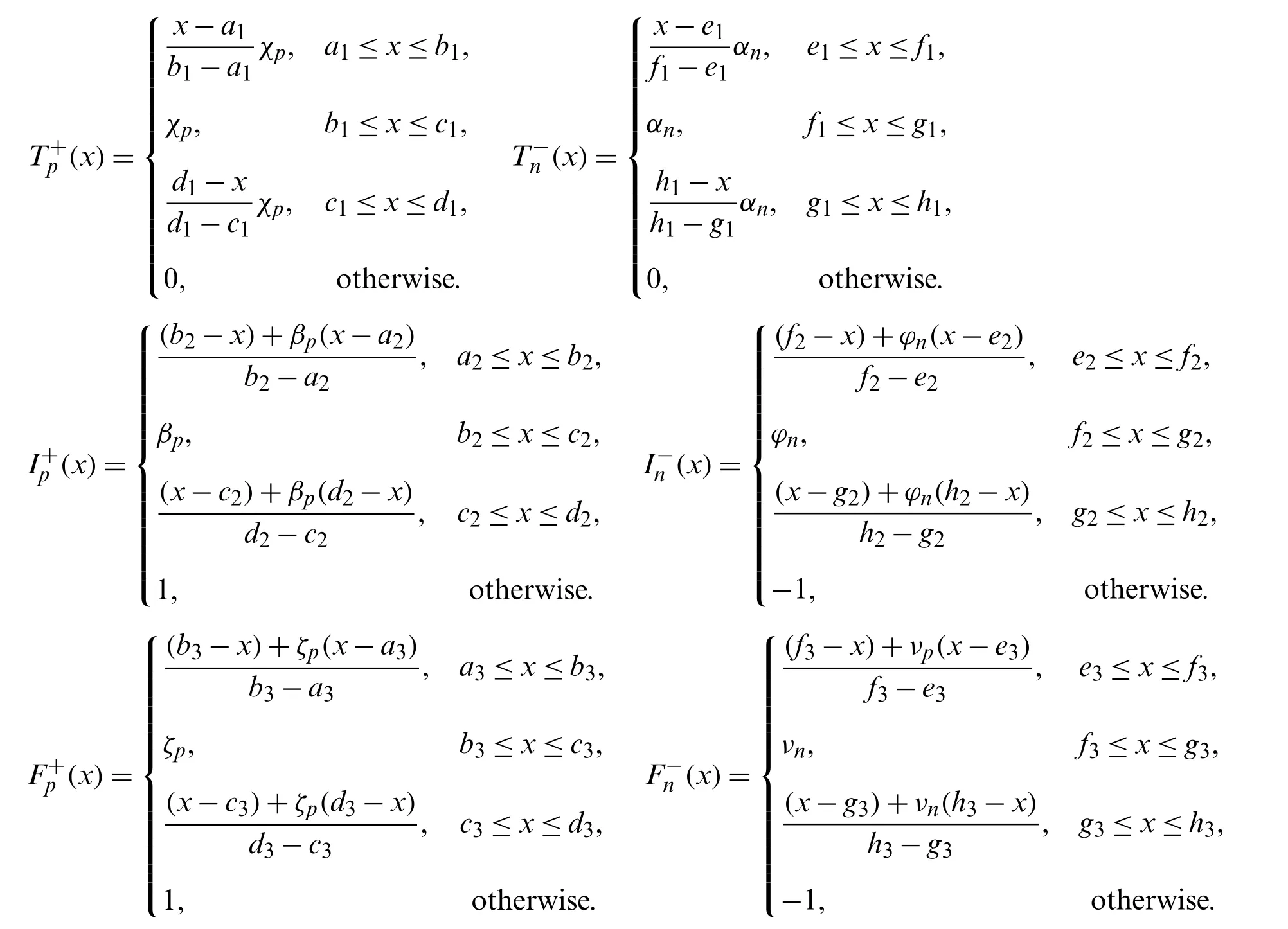
whereχp,βp,ζp∈[0,1] andαn,ϕn,νn∈[−1,0]⊂R.

Definition 2.9.Let

be two non-negativeTrBSvNNs, then

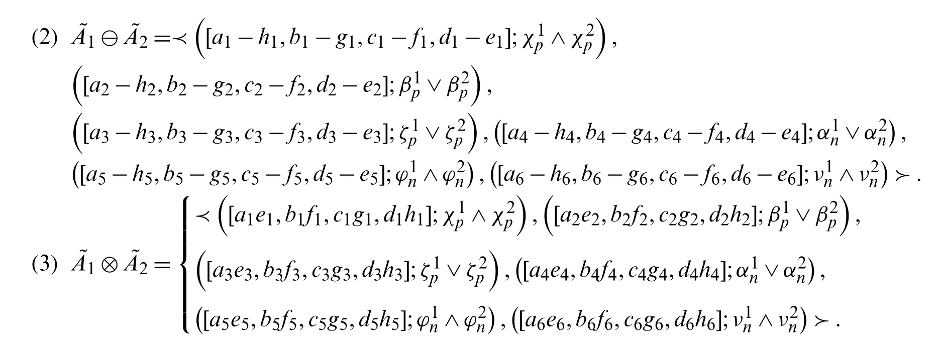
For other notations and applications, readers are referred to [43–45].

3 Methodology

In this section, a new method is presented to find the non-negative bipolar single-valued neutrosophic optimal solution ofFBSvNLPproblems with equality constraints, in which all the parameters are represented by non-negativeBSvNNs.

subject to

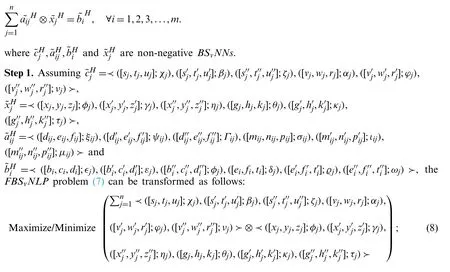
subject to

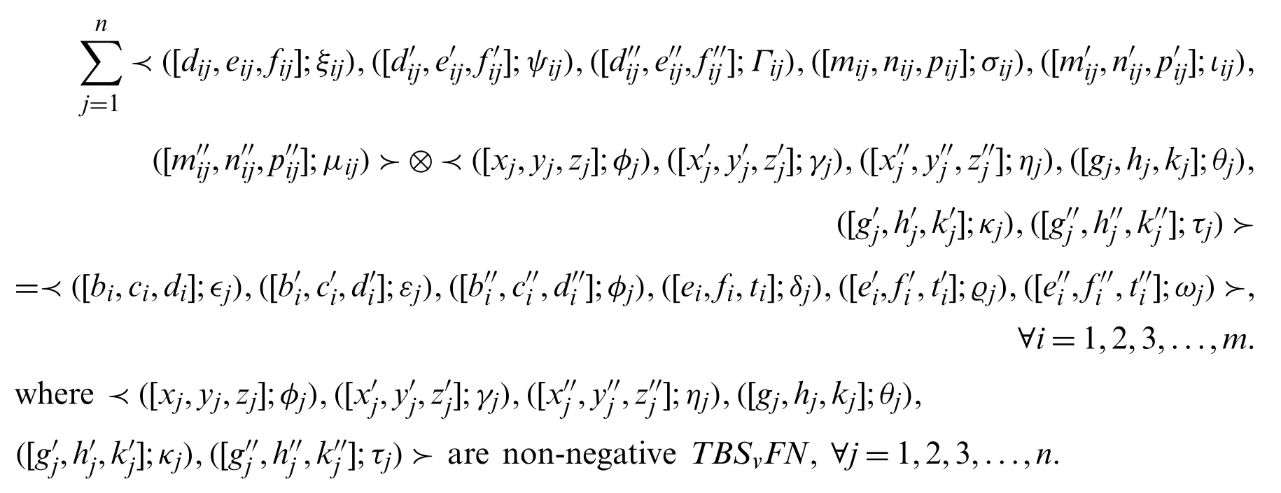
Step 2.Using product of non-negativeBSvNNs(2.9)and assuming

TheFBSvNLPproblem (8), can be transformed as follows:

subject to

Step 3.Using arithmetic operations (2.9), above problem becomes:

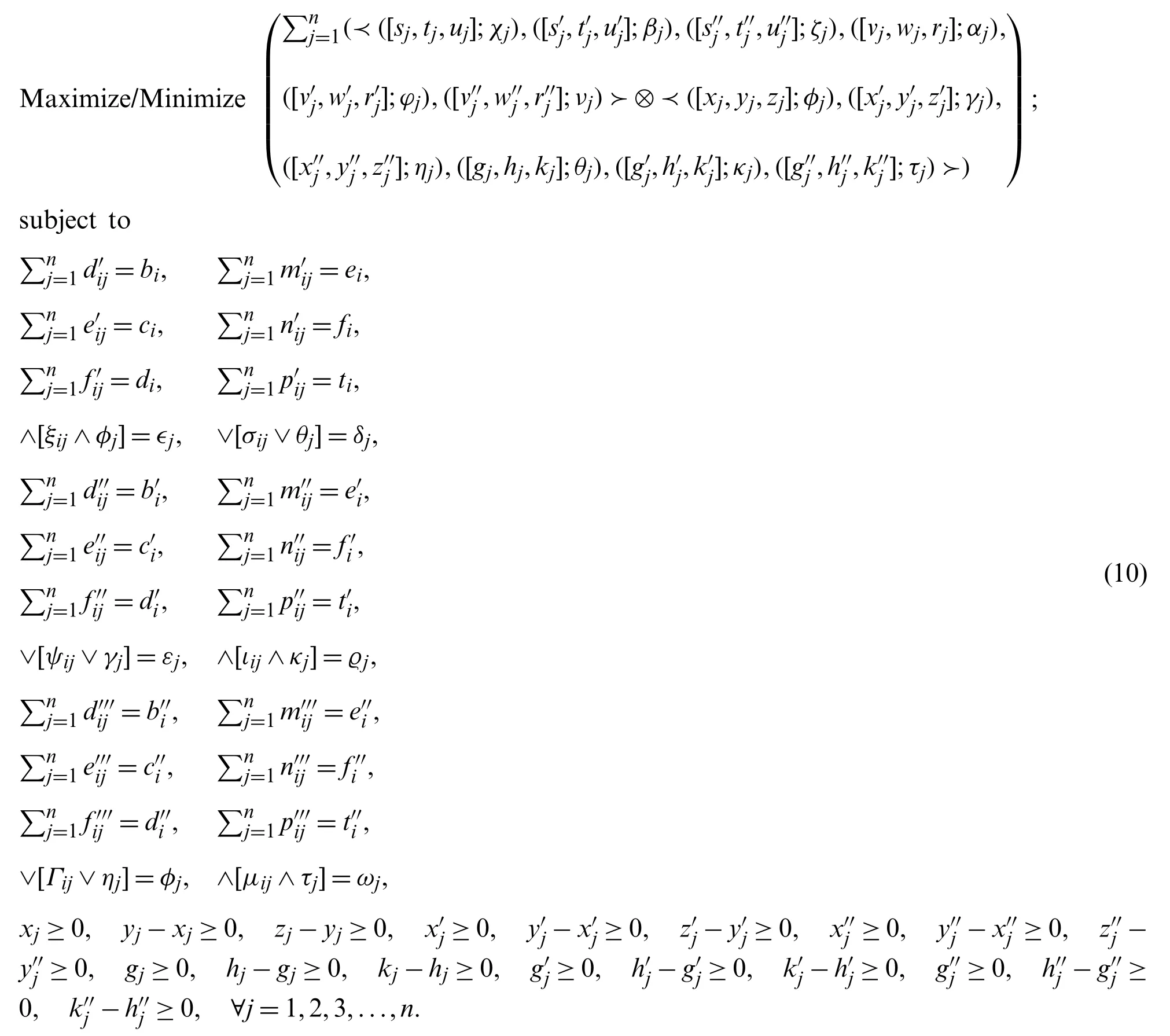
andφj,γj,ηj∈[0,1],θj,κj,τj∈[−1,0].

Step 4.By using score function (2.4), the neutrosophic optimal solution of theFBSvNLPproblem can be obtained by solving following CLP problem:

subject to:

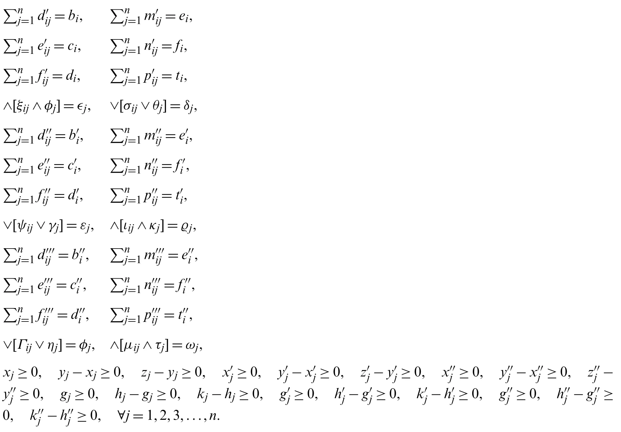
andφj,γj,ηj∈[0,1],θj,κj,τj∈[−1,0].

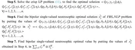
Thus, we state the existence condition for the optimal solution of bipolar single-valued neutrosophic LPP in the following Theorem:

Theorem 3.1.The solution of FBNLP problem

Maximize/Minimize

are non-negative TBNNs andare TBNNs exists, when the solution of the associated crisp LPP

Maximize/Minimize

subject to

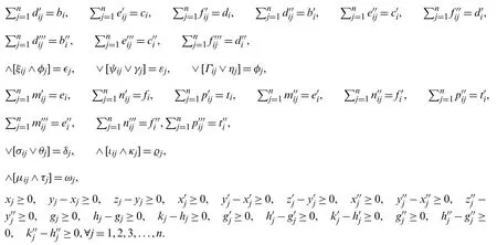
andφj,γj,ηj∈[0,1],θj,κj,τj∈[−1,0].

∀i=1,...,mexists.Otherwise, there is no guarantee that the bipolar single-valued neutrosophic optimal solution exists.

Proof.Straightforward.

4 Numerical Examples

In this section, we present numerical examples and models to illustrate the methodology given in Section 3.

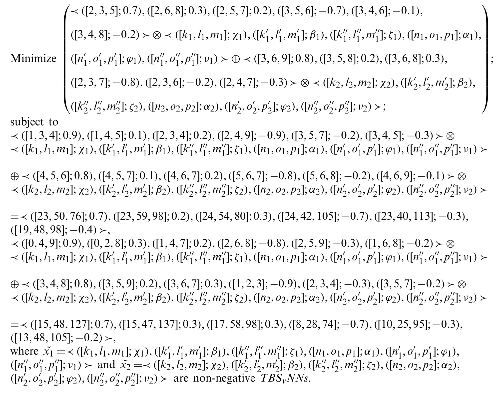
Example 4.1.Minimize ≺([2,3,5];0.7),([2,6,8];0.3),([2,5,7];0.2),([3,5,6];−0.7),([3,4,6];−0.1),([3,4,8];−0.2)≻⊗⊕≺([3,6,9];0.8),([3,5,8];0.2),([3,6,8];0.3),([2,3,7];−0.8),([2,3,6];−0.2),([2,4,7];−0.3)≻⊗

subject to

Step 1.

Step 2.

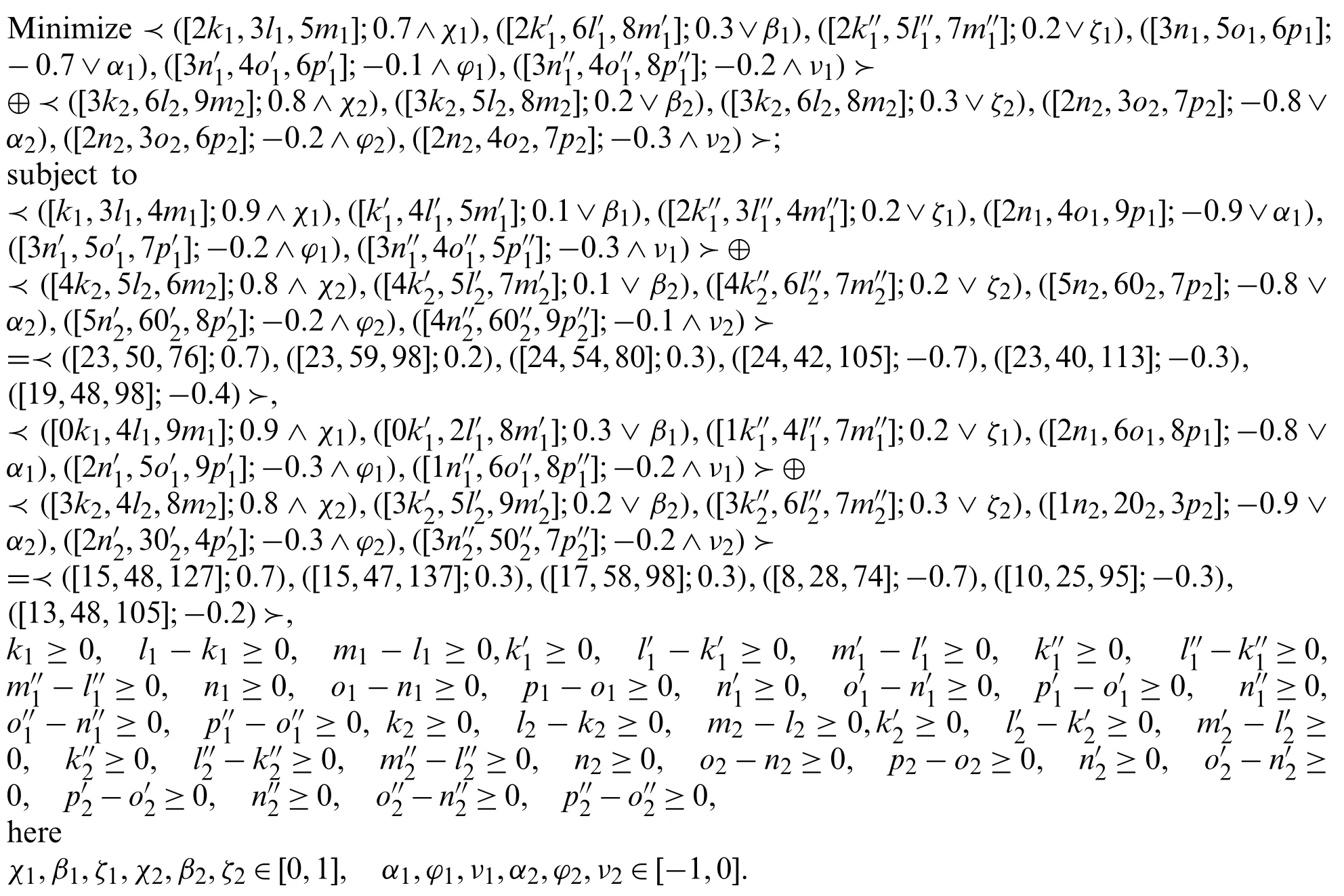
Step 3.

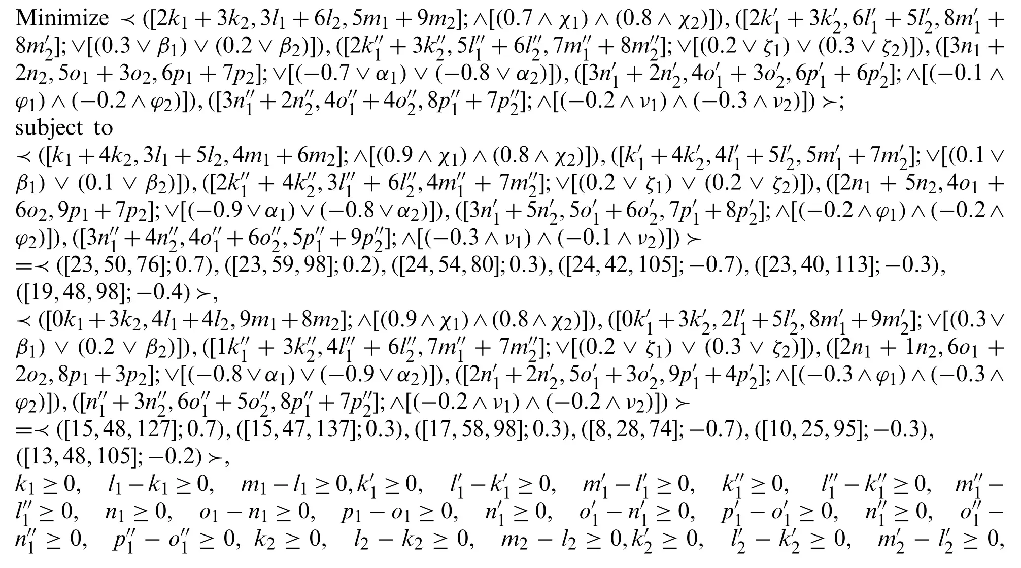
Step 4.

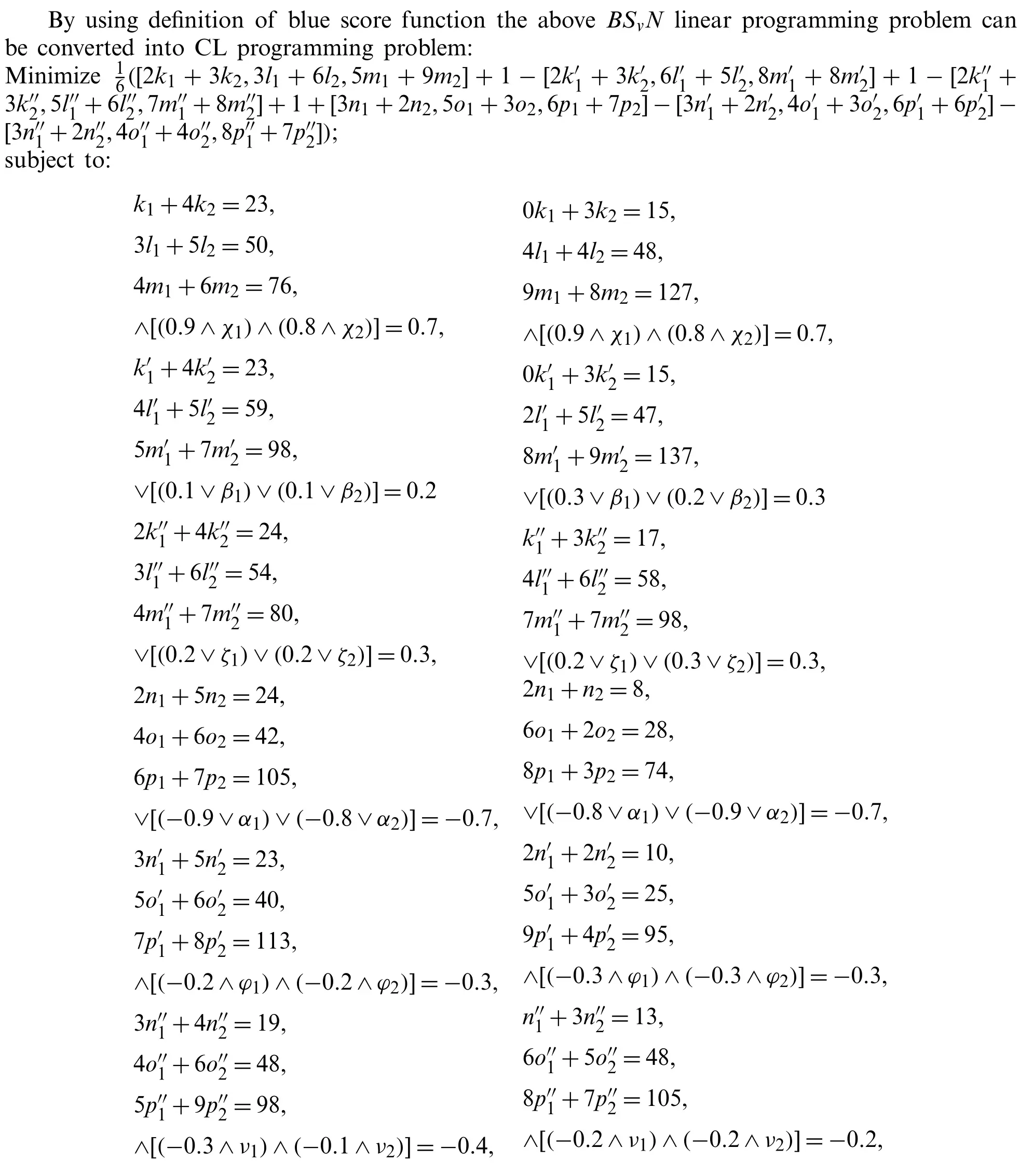
Step 5.

Step 6.

The exact optimal solution is=≺([3,5,7];0.8),([3,6,7];0.2),([2,4,6];0.3),([2,3,7];−0.8),([1,2,7];−0.3),([1,3,7];−0.2)≻,=≺([5,7,8];0.7),([5,7,9];0.2),([5,7,8];0.1),([4,5,6];−0.7),([4,5,8];−0.3),([4,6,9];−0.1)≻.

Step 7.

The bipolar single-valued neutrosophic optimal value of fully bipolar single-valued neutrosophic linear programming problem is≺([21,57,107];0.7),([21,71,128];0.3),([19,62,106];0.3),([14,30,84];−0.7),([11,23,90];−0.3),([11,36,119];−0.3)≻.

Example 4.2.Farming Problem.A farmer contains cattle like cows and goats in his form and he cells ghee and meat.The price of ghee per kg is Rs.≺([5,7,9];0.9,0.4,0.3),([6,7,8];−0.9,−0.1,−0.2)≻and for meat is Rs.≺([4,6,8];0.7,0.3,0.3),([3,7,9];−0.8,−0.4,−0.1)≻the maximum production of ghee is≺([7,17,38];0.8,0.4,0.4),([13,50,112];−0.7,−0.3,−0.4)≻kg per day and meat is≺([9,32,67];0.6,0.3,0.4),([14,48,120];−0.6,−0.3,−0.4)≻kg per day.The ghee and meat (in kg)of both cattle’s are given in Tab.1.

Table 1: Farming problem

We have to maximize the profit.Letandbe ghee and meat in kg.Then the bipolar single-valued neutrosophic linear programming problem becomes:Maximize ≺([5,7,9];0.9,0.4,0.3),([6,7,8];−0.9,−0.1,−0.2)≻⊗⊕≺([4,6,8];0.7,0.3,0.3),([3,7,9];−0.8,−0.4,−0.1)≻⊗

subject to

≺([2,3,5];0.9,0.4,0.2),([1,5,8];−0.7,−0.3,−0.1)≻⊗⊕≺([3,4,6];0.9,0.3,0.4),([4,5,7];−0.9,−0.2,−0.2)≻

≺([4,8,10];0.6,0.2,0.1),([2,4,8];−0.7,−0.2,−0.4)≻⊗⊕≺([1,4,9];0.7,0.1,0.1),([2,6,8];−0.6,−0.2,−0.2)≻

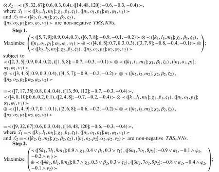
subject to

≺([2k1,3l1,5m1];0.9 ∧χ1,0.4 ∨β1,0.2 ∨ζ1),([1n1,5o1,8p1];−0.7 ∨α1,−0.3 ∧ϕ1,−0.1 ∧ν1)≻⊕

≺([3k2,4l2,6m2];0.9 ∧χ2,0.3 ∨β2,0.4 ∨ζ2),([4n2,502,7p2];−0.9 ∨α2,−0.2 ∧ϕ2,−0.2 ∧ν2)≻

=≺([7,17,38];0.8,0.4,0.4),([13,50,112];−0.7,−0.3,−0.4)≻,

≺([4k1,8l1,10m1]0.6 ∧χ1,0.2 ∨β1,0.1 ∨ζ1),([2n1,4o1,8p1];−0.7 ∨α1,−0.2 ∧ϕ1,−0.4 ∧ν1)≻⊕

≺([k2,4l2,9m2];0.7 ∧χ2,0.1 ∨β2,0.1 ∨ζ2),([2n2,602,8p2];−0.6 ∨α2,−0.2 ∧ϕ2,−0.2 ∧ν2)≻

=≺([9,32,67];0.6,0.3,0.4),([14,48,120];−0.6,−0.3,−0.4)≻,

k1≥0,l1−k1≥0,m1−l1≥0,n1≥0,o1−n1≥0,p1−o1≥0,

k2≥0,l2−k2≥0,m2−l2≥0,n2≥0,o2−n2≥0,p2−o2≥0,

here

χ1,β1,ζ1,χ2,β2,ζ2∈[0,1],α1,ϕ1,ν1,α2,ϕ2,ν2∈[−1,0].

Step 3.

Maximize ≺([5k1+4k2,7l1+6l2,9m1+8m2];∧[(0.9 ∧χ1)∧(0.7 ∧χ2)],∨[(0.4 ∨β1)∨(0.3 ∨β2)],

∨[(0.3 ∨ζ1)∨(0.3 ∨ζ2)]),([6n1+3n2,7o1+7o2,8p1+9p2];∨[(−0.9 ∨α1)∨(−0.8 ∨α2)],

∧[(−0.1 ∧ϕ1)∧(−0.4 ∧ϕ2)],∧[(−0.2 ∧ν1)∧(−0.1 ∧ν2)])≻;

subject to

≺([2k1+3k2,3l1+4l2,5m1+6m2];∧[(0.9 ∧χ1)∧(0.9 ∧χ2)],∨[(0.4 ∨β1)∨(0.3 ∨β2)],

∨[(0.2 ∨ζ1)∨(0.4 ∨ζ2)]),([n1+4n2,5o1+5o2,8p1+7p2];∨[(−0.7 ∨α1)∨(−0.9 ∨α2)],

∧[(−0.3 ∧ϕ1)∧(−0.2 ∧ϕ2)],∧[(−0.1 ∧ν1)∧(−0.2 ∧ν2)])≻

=≺([7,17,38];0.8,0.4,0.4),([13,50,112];−0.7,−0.3,−0.4)≻,

≺([4k1+k2,8l1+4l2,10m1+9m2];∧[(0.6 ∧χ1)∧(0.7 ∧χ2)],∨[(0.2 ∨β1)∨(0.1 ∨β2)],

∨[(0.1 ∨ζ1)∨(0.1 ∨ζ2)]),([2n1+2n2,4o1+6o2,8p1+8p2];∨[(−0.7 ∨α1)∨(−0.6 ∨α2)],

∧[(−0.2 ∧ϕ1)∧(−0.2 ∧ϕ2)],∧[(−0.4 ∧ν1)∧(−0.2 ∧ν2)])≻

=≺([9,32,67];0.6,0.3,0.4),([14,48,120];−0.6,−0.3,−0.4)≻,

k1≥0,l1−k1≥0,m1−l1≥0,n1≥0,o1−n1≥0,p1−o1≥0,

k2≥0,l2−k2≥0,m2−l2≥0,n2≥0,o2−n2≥0,p2−o2≥0,

here

χ1,β1,ζ1,χ2,β2,ζ2∈[0,1],α1,ϕ1,ν1,α2,ϕ2,ν2∈[−1,0].

Step 4.

By using definition of score function the aboveBSvNlinear programming problem can be converted into CL programming problem

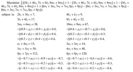
here

χ1,β1,ζ1,χ2,β2,ζ2∈[0,1],α1,ϕ1,ν1,α2,ϕ2,ν2∈[−1,0].

Step 5.

The optimal solution of the crisp linear programming problem isk1=2,l1=3,m1=4,k2=1,l2=2,m2=3,n1=5,o1=6,p1=7,n2=2,o2=4,p2=8,χ1=0.8,β1=0.3,ζ1=0.4,χ2=0.9,β2=0.2,ζ2=0.3,α1=−0.8,ϕ1=−0.2,ν1=−0.3,α2=−0.8,ϕ2=−0.3,ν2=−0.4.

Step 6.

The exact optimal solution is=≺([2,3,4];0.8,0.3,0.4),([5,6,7];−0.8,−0.2,−0.3)≻,=≺([1,2,3];0.9,0.2,0.3),([2,4,8];−0.8,−0.3,−0.4)≻.

Step 7.

The bipolar single-valued neutrosophic optimal value of fully bipolar single-valued neutrosophic linear programming problem is:

≺([14,33,60];0.7,0.4,0.4),([36,70,128];−0.8,−0.4,−0.4)≻.

Example 4.3.Maximize Profit Problem.A company contains two plants namely, plant X and plant Y.It produces two products mobiles and LCDs by using raw material.The maximum working capacity for plant X is ≺([24,81,131,190];0.4,0.6,0.5),([24,66,128,229];−0.4,−0.6,−0.5)≻hrs per week and for plant Y is ≺([20,71,134,196];0.5,0.6,0.5),([44,90,152,218];−0.5,−0.6,−0.6)≻hrs per week.

For maximum production of mobiles and LCDs the raw material are given in Tab.2.

Table 2: Maximize profit problem

The cost of each mobile Rs.≺([5,7,9,11];0.5,0.4,0.3),([6,8,10,12];−0.6,−0.4,−0.5)≻and LCD Rs.≺([5,8,11,14];0.6,0.5,0.5),([7,9,11,13];−0.7,−0.5,−0.6)≻.How can the company maximize the profit by producing mobiles and LCDs in the market.Letandbe the production of mobiles and LCDs in h.

Then the bipolar single-valued neutrosophic linear programming problem becomes:

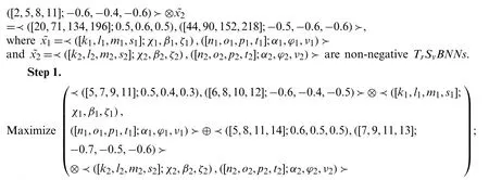
subject to

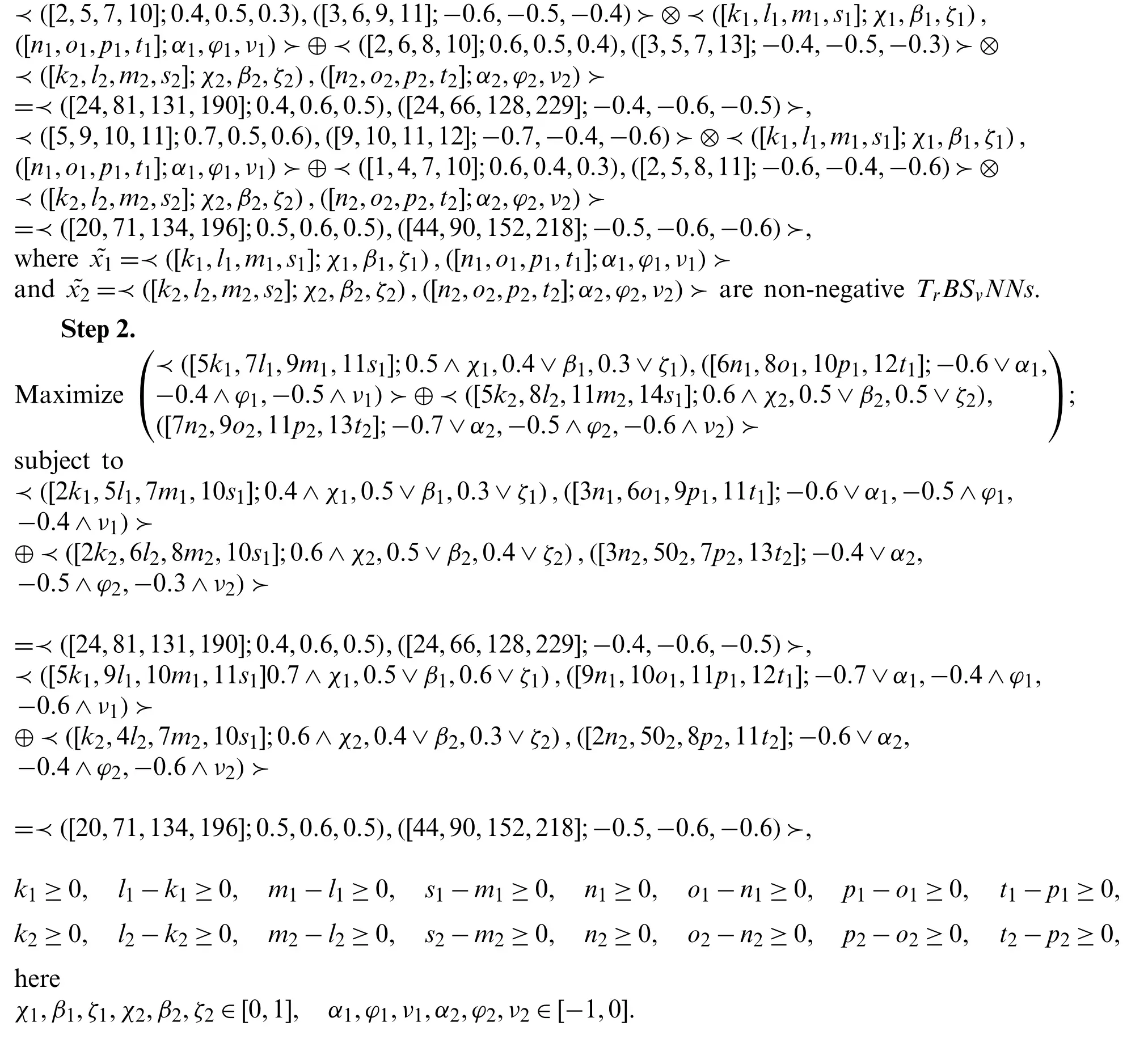
Step 3.

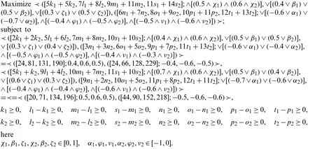
Step 4.

here

χ1,β1,ζ1,χ2,β2,ζ2∈[0,1],α1,ϕ1,ν1,α2,ϕ2,ν2∈[−1,0].

Step 5.

The optimal solution of the crisp linear programming problem isk1=2,l1=3,m1=5,s1=6,k2=10,l2=11,m2=12,s2=13,n1=4,o1=6,p1=8,t1=9,n2=4,o2=6,p2=8,t2=10,χ1=0.5,β1=0.6,ζ1=0.4,χ2=0.7,β2=0.6,ζ2=0.5,α1=−0.7,ϕ1=−0.4,ν1=−0.5,α2=−0.5,ϕ2=−0.6,ν2=−0.4.

Step 6.

The exact optimal solution is=≺([2,3,5,6];0.5,0.6,0.4),([4,6,8,9];−0.7,−0.4,−0.5)≻,=≺([10,11,12,13];0.7,0.6,0.5),([4,6,8,10];−0.5,−0.6,−0.4)≻.

Step 7.

The bipolar single-valued neutrosophic optimal value of fully bipolar single-valued neutrosophic linear programming problem is

≺([60,89,177,248];0.5,0.6,0.5),([52,102,168,238];−0.5,−0.6,−0.6)≻.

Step 2.

subject to

≺([3k1,5l1,6m1,8s1];0.6 ∧0.8,0.5 ∨0.2,0.4 ∨0.3),([9n1,10o1,11p1,12t1];−0.7 ∨−0.6,−0.5 ∧−0.4,

−0.3 ∧−0.4)≻⊕≺([5k2,8l2,10m2,14s2];0.3 ∧0.8,0.6 ∨0.2,0.6 ∨0.3),([7n2,9o2,11p2,13t2];−0.4 ∨

−0.6,−0.5 ∧−0.4,−0.6 ∧−0.4)≻

=≺([18,42,68,116];0.3,0.6,0.6),([73,96,154,200];−0.4,−0.5,−0.6)≻,

≺([5k2,8l2,10m2,14s2];0.3 ∧0.8,0.6 ∨0.2,0.6 ∨0.3),([7n2,9o2,11p2,13t2];−0.4 ∨−0.6,−0.5 ∧

−0.4,−0.6 ∧−0.4)≻⊕≺([3k1,5l1,6m1,8s1];0.6 ∧0.8,0.5 ∨0.2,0.4 ∨0.3),([9n1,10o1,11p1,12t1];

−0.7 ∨−0.6,−0.5 ∧−0.4,−0.3 ∧−0.4)

=≺([14,36,60,104];0.3,0.6,0.6),([71,114,154,200];−0.4,−0.5,−0.6)≻,

k1≥0,l1−k1≥0,m1−l1≥0,s1−m1≥0,n1≥0,o1−n1≥0,p1−o1≥0,t1−p1≥0,

k2≥0,l2−k2≥0,m2−l2≥0,s2−m2≥0,n2≥0,o2−n2≥0,p2−o2≥0,t2−p2≥0,

Step 3.

Maximize ≺([3k1+5k2,5l1+8l2,6m1+10m2,8s1+14s2];∧[(0.6 ∧0.8)∧(0.3 ∧0.8)],∨[(0.5 ∨0.2)∨(0.6 ∨0.2)],

∨[(0.4∨0.3)∨(0.6∨0.3)]),([9n1+7n2,10o1+9o2,11p1+11p2,12t1+13t2];∨[(−0.7∨−0.6∨(−0.4∨−0.6)],∧[(−0.5 ∧−0.4)∧(−0.5 ∧−0.4)],∧[(−0.3 ∧−0.4)∧(−0.6 ∧−0.4)])≻;

subject to

≺([3k1+5k2,5l1+8l2,6m1+10m2,8s1+14s2];∧[(0.6 ∧0.8)∧(0.3 ∧0.8)],∨[(0.5 ∨0.2)∨(0.6 ∨0.2)],

∨[(0.4∨0.3)∨(0.6∨0.3)]),([9n1+7n2,10o1+9o2,11p1+11p2,12t1+13t2];∨[(−0.7∨−0.6∨(−0.4∨

−0.6)],∧[(−0.5 ∧−0.4)∧(−0.5 ∧−0.4)],∧[(−0.3 ∧−0.4)∧(−0.6 ∧−0.4)])≻

=≺([18,42,68,116];0.3,0.6,0.6),([73,96,154,200];−0.4,−0.5,−0.6)≻,

≺([5k1+3k2,8l1+5l2,10m1+6m2,14s1+8s2];∧[(0.3 ∧0.8)∧(0.6 ∧0.8)],∨[(0.6 ∨0.2)∨(0.5 ∨0.2)],

∨[(0.6∨0.3)∨(0.4∨0.3)]),([7n1+9n2,9o1+10o2,11p1+11p2,13t1+12t2];∨[(−0.4∨−0.6)∨(−0.7∨

−0.6)],∧[(−0.5 ∧−0.4)∧(−0.5 ∧−0.4)],∧[(−0.6 ∧−0.4)∧(−0.3 ∧−0.4)])≻

=≺([14,36,60,104];0.3,0.6,0.6),

([71,114,154,200];−0.4,−0.5,−0.6)≻,

k1≥0,l1−k1≥0,m1−l1≥0,s1−m1≥0,n1≥0,o1−n1≥0,p1−o1≥0,t1−p1≥0,

k2≥0,l2−k2≥0,m2−l2≥0,s2−m2≥0,n2≥0,o2−n2≥0,p2−o2≥0,t2−p2≥0,

Step 4.

By using definition of score function the aboveBSvNlinear programming problem can be converted into CL programming problem

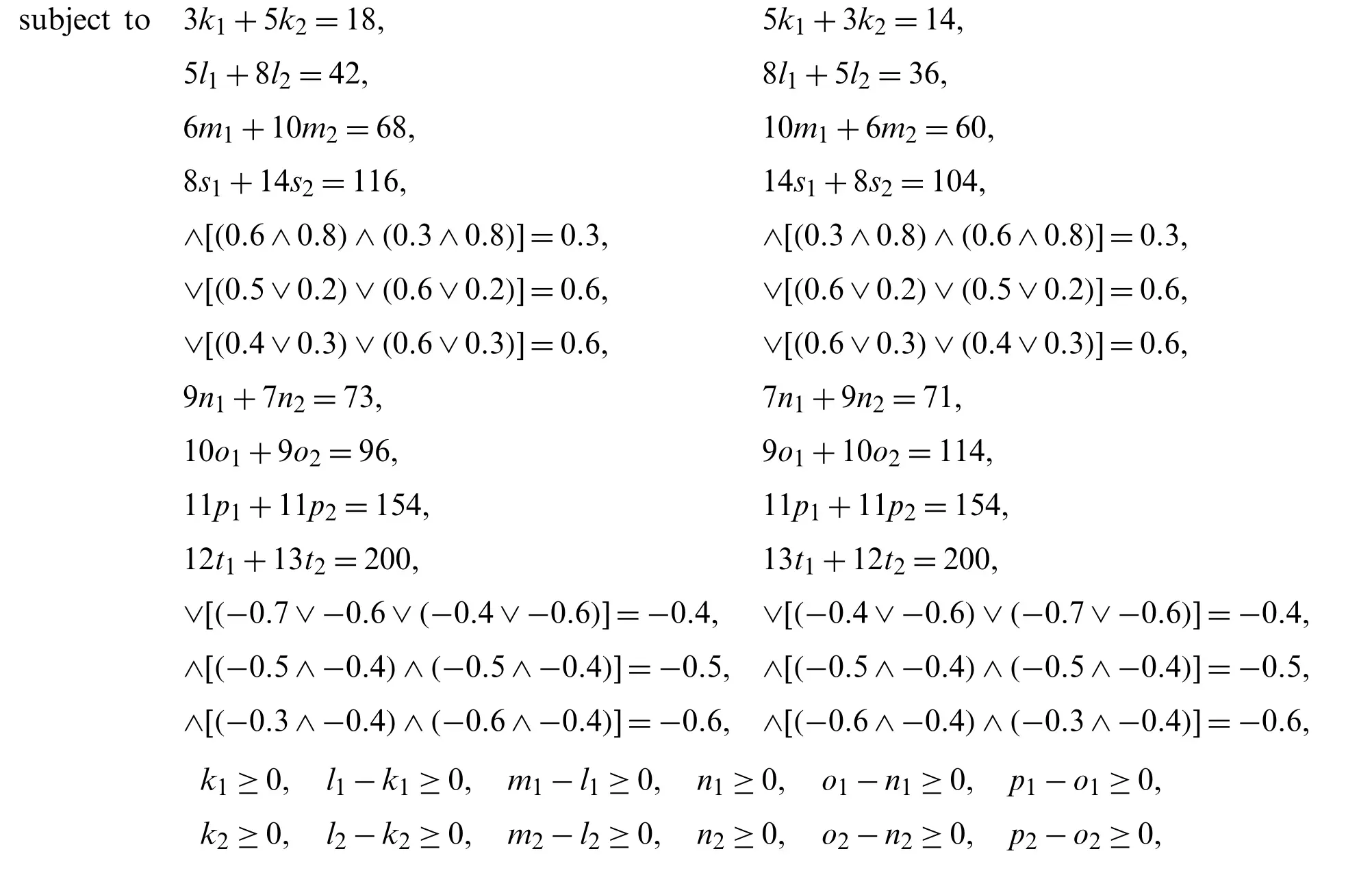
Step 5.

The optimal solution of the crisp linear programming problem isk1=1,l1=2,m1=3,s1=4,k2=3,l2=4,m2=5,s2=5,n1=5,o1=6,p1=7,t1=8,n2=4,o2=6,p2=7,t2=8.

Step 6.

The exact optimal solution is=≺([1,2,3,4];0.8,0.2,0.3),([5,6,7,8];−0.6,−0.4,−0.4)≻,=≺([3,4,5,6];0.8,0.2,0.3),([4,6,7,8];−0.6,−0.4,−0.4)≻.

Step 7.

The bipolar single-valued neutrosophic optimal value of fully bipolar single-valued neutrosophic linear programming problem is≺([18,42,68,116];0.3,0.6,0.6),([73,96,154,200];−0.4,−0.5,−0.6)≻.

5 Comparative Analysis

In this section, Khalifa et al.’s method [38] has been compared with our proposed method in Section 3.Bipolar single-valued neutrosophic optimal solution of the Example (4.4)is=≺([1,2,3,4];0.8,0.2,0.3),([5,6,7,8];−0.6,−0.4,−0.4)≻,=≺([3,4,5,6];0.8,0.2,0.3),([4,6,7,8];−0.6,−0.4,−0.4)≻and bipolar single-valued neutrosophic optimal value ≺([18,42,68,116];0.3,0.6,0.6),([73,96,154,200];−0.4,−0.5,−0.6)≻.By restricting the bipolarity membership part of Example (4.4), the problem converts into FNLP problem;

subject to

≺([3,5,6,8];0.6,0.5,0.4)≻⊗⊕≺([5,8,10,14];0.3,0.6,0.6)≻⊗

=≺([16,18,22,30];0.8,0.2,0.3)≻,

≺([5,8,10,14];0.3,0.6,0.6)≻⊗⊕≺([3,5,6,8];0.6,0.5,0.4)≻⊗

=≺([13,15,18,24];0.8,0.2,0.3)≻,

Neutrosophic optimal solution and neutrosophic optimal value attained by Khalifa et al.’s method [38] are=([3.3,4,4.6,6];0.8,0.2,0.3)=([6.3,7,8.3,12];0.8,0.2,0.3)and([41.4,78,119,220.8];0.3,0.6,0.6), respectively.These values ofandhave been not satisfied the constraints.So, our proposed method is accurately solved tha Khalifa et al.’s [38].problem in an bipolar single-valued neutrosophic environment and satisfied the constraints.

Furthermore, our proposed method is generalization of Khalifa et al.’s [38] method by using this method all the shortcoming of Khalifa et al.’s [38] method are removed.

6 Conclusions

A bipolar single-valued neutrosophic model, an extension of bipolar fuzzy model, is a powerful tool to deal with vagueness.In this research article, we have solved fully bipolar single-valued neutrosophic linear programming problems with equality constraints.We have applied a score function to transform bipolar single-valued neutrosophic numbers into its equivalent crisp problem.Further, we have solved the numerical examples and practical models by using the proposed method.The obtained solutions satisfy the given constraints of the FBSvNLP problems, which shows that the suggested method is reliable.In future, this work can be extended to (1)Complex bipolar neutrosophic LPP; (2)Complex spherical neutrosophic LPP.

Funding Statement:The authors did not receive financial support for the research.

Conflicts of Interest:The authors declare that they have no conflicts of interest to report regarding the present study.