A Two-plume Convective Model for Precipitation Extremes

Zihan YIN, Panxi DAI, and Ji NIE

Department of Atmospheric and Oceanic Sciences, School of Physics, Peking University, Beijing 100029, China

ABSTRACT

Key words:precipitation extremes, convective model, rain evaporation, environmental descent

1.Introduction

Understanding the dynamics of precipitation extremes(heavy precipitation events) and their responses to climate change is of great importance. Water vapor condensation and precipitation, by their nature, occur at cloud-microphysical and convective scales; however, the commonly used meteorological variables in global climate models (GCMs) are usually large-scale variables representing the grid-mean properties of tens-to-hundreds of kilometers scales (referred to as the GCM-grid scale in this study). Thus, an essential step in diagnosing the precipitation extremes in GCMs is to adopt a simple model relating precipitation with the GCMgrid-mean variables, typically including a thermodynamic variable representing atmospheric moisture and a dynamic variable representing large-scale vertical motion. These simple models (e.g., Emori and Brown, 2005; O’Gorman and Schneider, 2009a, b; Sugiyama et al., 2010; Chen et al.,2019) have been proven valuable in studies of precipitation extremes in several aspects, such as examining the coupling between large-scale and convective-scale dynamics in precipitation extremes (Nie et al., 2016; Nie and Fan, 2019),decomposing the thermodynamic and dynamic controls of precipitation extremes (O’Gorman and Schneider, 2009a;Seager et al., 2012; Pfahl et al., 2017; Li and O’Gorman,2020; Nie et al., 2020), and identifying uncertainties and model spreads among GCM simulations (O’Gorman and Schneider, 2009b; Sugiyama et al., 2010).

A good simple model for precipitation extremes shall meet two requirements. First, the physical picture upon which the model is built depicts the relevant processes. In that case, the model also provides valuable insights into our understanding of the system. Second, the model results in a reasonably accurate approximation of precipitation extremes, so it is practically useful. In addition to the two requirements, a model with a simple formula and commonly used large-scale variables is favored. The previously proposed simple models of precipitation extremes may be classified into two categories based on their physical arguments. Models in the first category (e.g., Emori and Brown,2005; Westra et al., 2013; Nie et al., 2018; Chen et al.,2019) are based on the column moisture budget. Alternatively, O’Gorman and Schneider (2009a, b) proposed a model (the second-category model) based on saturated ascending air during heavy rainfall, and this model has enjoyed more popularity over recent years. The first-category models neglect the source and sink terms of moisture, and the key assumption of the second-category model that the whole air column is homogeneous and saturated may be oversimplified. Both models have sizeable errors in reproducing extreme precipitation climatology in many regions (e.g.,Pfahl et al., 2017).

In this study, we propose a two-plume convective model for precipitation extremes with improved physical bases and accuracy. This model takes the sub-GCM-grid inhomogeneity of convection into account. It uses two plumes to model the precipitation extremes: one for convective updrafts and one for the unsaturated environment. The paper is organized as follows: In section 2, we introduce the data and two previously proposed models and show that these two models have sizeable errors in reproducing precipitation extremes in climate simulations. In section 3, we evaluate the sub-GCM-grid inhomogeneity using high-resolution observational data (reanalysis), introduce the two-plume convective model, and demonstrate its improvement in the estimation of extreme precipitation. Conclusions and discussion are presented in section 4.

2.Data and models

2.1.Data

The GCMs differ substantially from each other in many aspects; to avoid dependences of results on individual GCMs, we evaluate the simple models of precipitation extremes using 20 GCM outputs in the CMIP5 achieve(Coupled Model Intercomparison Project Phase 5, Table S1 in the Electronic Supplementary Material, ESM). The outputs are daily data of the historical simulations between 1981 and 2000. The outputs of the 20 GCMs are interpolated to a 2.5° × 2.5° geographical grid so that they have the same horizontal resolution. The variables include pressure velocity ( ω), temperature ( T ), specific humidity ( q) and relative humidity ( r ) on vertical pressure ( p) levels, and surface precipitation. In GCMs, precipitation (and convection) is usually parameterized by several modules (e.g., convective precipitation produced by the convective parameterization of cumulus clouds, and grid-scale precipitation produced by the parameterization of stratus or layered clouds). This separation is an ad hoc treatment due to the insufficient resolution of GCMs. In this study, convection refers to clouds of all types.

The precipitation extreme examined in this study is defined as the annual maximum daily precipitation (i.e.,RX1day in the literature, Alexander et al., 2006, Pfahl et al.,2017; Nie et al., 2020). This definition is roughly equivalent to the 99.7th percentile of precipitation, close to the 99.9th percentile in some other previous studies (e.g., O’Gorman and Schneider, 2009a, b). As the threshold of precipitation extreme changes, the performances of the simple models vary, however, our conclusions are still valid (later see section 3.3). To obtain a better physical understanding of the full probability distribution of precipitation is important(e.g., Chen et al., 2019); however, it is beyond the scope of this study.

For the historical simulations, on each geographic grid we may find 20 extreme events (during the 20 years simulations) and their composites. We also extract the atmospheric variables conditioned on the extreme precipitation days, which are the inputs of the simple models. The precipitation extremes provided by the simple models are then compared with precipitation extremes from the direct outputs of GCMs. Their differences are treated as the errors of the simple models. The global mean relative error is the global sum of the absolute values of differences on each grid divided by the global sum of precipitation extremes. Unless otherwise specified, the results of the GCM outputs only show their multimodel means.

We use the high-resolution ERA-Interim reanalysis(Dee et al., 2011) as the observational basis to examine the sub-GCM-grid inhomogeneity of precipitation extremes.The ERA reanalysis provides daily data between 1979 and 2016, with a horizontal resolution of 0.25° × 0.25°. The ERA precipitation is from the short-range forecast, which shows reasonable agreement with those of the satellite- and rain gauge-based GPCP (Global Precipitation Climatology Project version 1.2; Huffman et al., 2001) precipitation (Dai and Nie, 2020). To match the resolution of the GCM outputs, we constructed a set of coarsened-resolution reanalyses (2.5° × 2.5°) based on the high-resolution (0.25° ×0.25°) reanalyses. Precipitation extremes are selected using the coarsened-resolution reanalyses, while the high-resolution reanalyses provide information on the sub-GCM-grid inhomogeneity.

2.2.Two previously proposed models

For precipitation extremes within an area of a typical GCM grid, previous models may be roughly divided into two categories. Models in the first category (named model 1, e.g., Emori and Brown, 2005) are based on the column moisture budget. Since in heavy precipitation events the moisture sink due to precipitation is mainly balanced by vertical moisture advection, model 1 approximates precipitation extremes ( P) as

where the overline denotes GCM-grid-mean variables, and{} denotes the vertical integral from the surface level to the tropopause (here defined as the layer where the pressure level below 50 hPa has a lapse rate of 2 K km−1). The subscript in P1denotes the model number (the same applies to model 2 and model 3). The variables in the simple models are conditioned on the extreme precipitation day. In model 1, the budget terms of moisture storage, horizontal moisture advection, surface evaporation, and moisture flux at the tropopause are neglected.

The second-category model (model 2, O’Gorman and Schneider, 2009a, b) suggests that during heavy rainfall, the air column is close to saturation. Thus, precipitation is the excess of water vapor of saturated rising air following moist adiabatic processes, which has the formula of

The above evaluation shows that model 1 and model 2 both have sizeable errors. Model 2 has better performance than model 1 has; however, it still has large errors in many regions. Over a GCM-grid-size column, saturated convective updrafts only occupy a fraction of area; saturation throughout the whole column is very rare even during heavy precipitation. Figure. S3 shows composites of relative humidity during precipitation extremes at several representative latitudes. Relative humidity during precipitation extremes can only reach up to approximately 70%-90% in the troposphere. Actually, many GCMs set an upper limit on the grid’s relative humidity by including a large-scale condensation parameterization. In the following, we propose a twoplume convective model for precipitation extremes that takes the sub-GCM-grid inhomogeneity into account and shows its improved performance.

Fig. 1. (a) Multimodel-mean climatology of precipitation extremes from the direct GCM outputs ( P0) in the CMIP5 historical simulations. (b) and (c) show the errors of model 1 and model 2 in reproducing precipitation extremes,respectively.

Table 1. The global-mean relative errors of the simple models.The time period for the RCP8.5 simulations is between 2081 and 2100. Note the global mean value of precipitation extreme is 22.8 mm d−1 for the CMIP5 historical simulations and 27.9 mm d−1 for the RCP8.5 simulations.

3.Results

3.1.The sub-GCM-grid inhomogeneity of precipitation extremes

The horizontal scale of convection is usually much smaller than that of typical GCM grids. During heavy precipitation events, condensation and precipitation are associated with only convective updrafts within the GCM grids. Model 2 essentially approximates the precipitation extremes with a homogenously saturated convective plume, neglecting the effects of the sub-GCM-grid inhomogeneity.

We evaluate the sub-GCM-grid inhomogeneity of precipitation extremes by comparing the ERA reanalyses of high and coarsened resolutions. At each geographic location, 38 precipitation extremes (one event each year between 1979 and 2016) are selected from the coarsened-resolution reanalysis. Then, we examine the statistics of high-resolution data within the coarsened grids. Convective updrafts are defined as high-resolution grids with ω >0.1 Pa s−1at 500 hPa,and the rest are defined as environmental air. The following analyses are not sensitive to the definition. For example,slightly changing the threshold or using a different criterion,such as liquid water content greater than a threshold, leads to similar conclusions. Next, we calculate the convective updraft coverage ( a, fractional area of convective updrafts within a coarsened-resolution grid) and the mean properties of convective updrafts (denoted by subscript c) and environmental air (denoted by subscript e) of precipitation extremes.

Figure 2 shows the map of convective updraft coverage during precipitation extremes. It is clear that within a GCM-scale grid, only a fraction of areas are convective updrafts during precipitation extremes, consistent with the relative humidity profile shown in Fig. S2. The probability distribution of a peaks around a =0.6, while events with a close to 1 or 0 are rare. There are distinct geographic patterns of a. Regions with greater climatology of precipitation extremes have a values closer to 1 (Figs. 1a and 2), while regions with weaker precipitation extremes have smaller a values.

The dynamic and thermodynamic properties of convective updrafts and the coarsened-resolution grid means are compared for different a bins in Fig. 3. Convective updrafts are moister than the grid means (Fig. 3a), consistent with the fact that the gird mean humidity is not saturated (Fig. S2).As expected, the moisture difference increases asa decreases. In contrast, the temperature difference between the convective updrafts and the grid means is very small regardless of a (Fig. 3b). This slight temperature difference is also found in cloud observations from aircraft (e.g., Austin et al., 1985) and cloud-resolving simulations (e.g., Singh and O'Gorman, 2013). In many convective parameterizations, this small temperature difference is neglected (also called the zero-buoyancy approximation, Bretherton and Park, 2008; Singh and O'Gorman, 2013; Nie et al., 2019).The zero-buoyancy approximation states that any sizeable buoyancy difference between cloudy and environmental air will lead to strong entrainment mixing that consumes the positive buoyancy of clouds. Figure 3c shows that the convective updrafts have much greater vertical velocity than the grid means. These results indicate that using the grid means or, equivalently, a homogeneous plume to represent precipitation extremes may lead to systematic biases.

3.2.A two-plume convective model for precipitation extremes

Fig. 2. Geographic distribution of the convective updraft coverage during precipitation extremes from the ERA reanalysis.

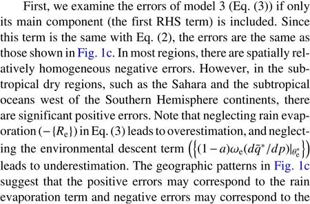
There are three components, cloud condensation (the dominant component), environmental motion, and rain evaporation, corresponding to the right-hand-side (RHS) terms in Eq. (3), respectively. The condensation term shares the same formula as that of model 2 (Eq. (2)); however, the interpretations of the two models are different. The other two components, environmental motion and rain evaporation, are secondary in terms of the global mean; however, they may be significant regionally.

The two-plume convective model provides a new physical picture relating heavy precipitation, convection, and large-scale variables (see the schematic in Fig. 4). The previously proposed model 2 is based on the picture of columnwise ascent of horizontal homogenous saturated air. Here,the two-plume model highlights inhomogeneity within the air column: condensation and precipitation are only associated with convective updrafts occupying a part of the column, the environmental air is unsaturated and its vertical motion also contributes to the column means. The twoplume model does not require column-wise saturation, thus resolving the conflict between the saturation assumption in model 2 and the GCM outputs.

3.3.Improvement of the convective model

In this subsection, we parameterize the two sub-GCMgrid processes in model 3, rain evaporation and environmental motion, using the grid mean variables and show improvement of the convective model (model 3) in reproducing precipitation extremes.

Fig. 4. Schematic of the two-plume convective model for precipitation extremes. Note the convective updrafts represent convection parameterized by both the convective parameterization module and grid-scale condensation module in GCMs.

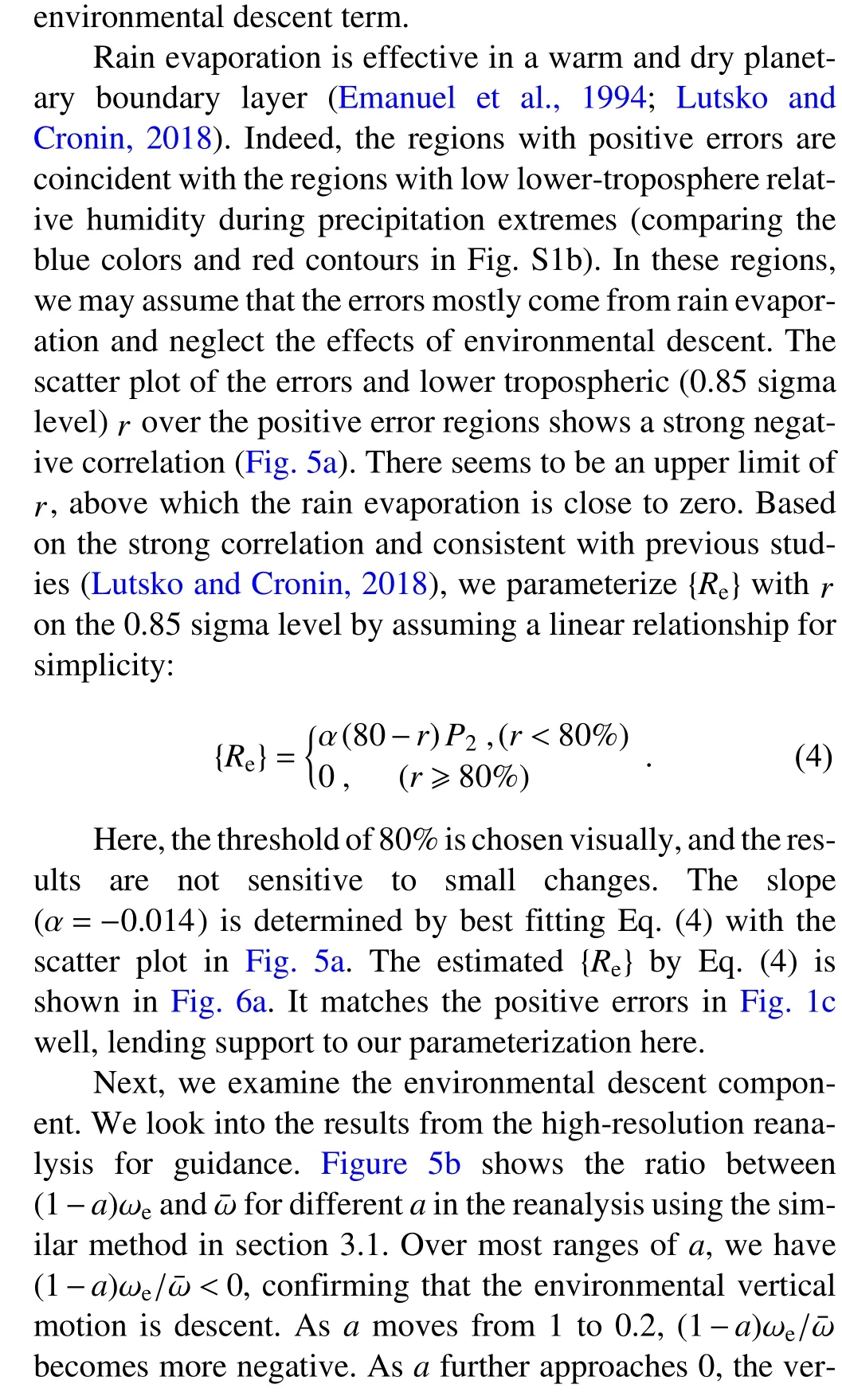
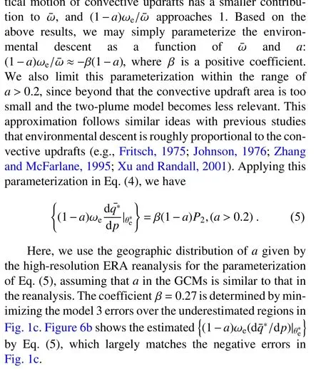
With the above empirical parameterization of rain evaporation and environmental descent, the two-plume convective model reproduces the climatology of precipitation extremes quite well (Figs. 6c and S1c). It reduces the global mean error by approximately half from model 2 (from 10.6% to 5.5%, Table 1), and largely reduces regional errors. The two-plume model not only works for the multimodel means,but also improves individual GCMs. For each GCM, its fitting parameters in Eqs. (4) and (5) are slightly different from the parameters for the multimodel means (Fig. S4a),due to the internal differences among the GCMs. The improvement of model 3 for each GCM output is also substantial (Fig. S4b). We also tested the sensitivity of our results on the threshold of precipitation extremes. For less intense precipitation extremes, model 3 still shows significant improvement over the other two models (Fig. S5). These comparisons indicate that the parametrizations of the two additional physical processes in the two-plume model are robust.

The convective model also works well for different climates, such as a warmer climate. We apply similar evaluations for the CMIP5 RCP8.5 simulations between 2081 and 2100. With the same parameters used for the historical simulations, model 3 has a global mean relative error of 5.4%, much smaller than that of model 2 (11.5%, Table 1).Again, model 3 reduces the regional errors significantly(Fig. S6). We calculated the parameters in Eqs. (4) and (5)by fitting them using the outputs of the RCP8.5 simulations.They are very close to the parameters obtained in the historical simulations, and the performance of model 3 is very close regardless of which set of parameters is used. This comparison indicates that the parametrizations of the two additional physical processes in the convective model are robust and likely reliable for different climates.

4.Conclusions and discussion

This study proposes a two-plume convective model that approximates precipitation extremes with large-scale (i.e.,GCM-grid-mean) variables. The convective model is built upon a physical picture in which the precipitating regional column consists of convective updrafts and unsaturated environments (Fig. 4) and includes three components: cloud condensation, rain evaporation, and environmental descent. The three components are expressed or parameterized using GCM-grid-mean variables with the zero-buoyancy approximation and guidance from the high-resolution reanalysis. The model is evaluated using outputs from 20 CMIP5 GCM simulations and compared with two previously proposed and widely used models. The new model largely reduces errors in reproducing precipitation extremes in terms of both global mean and regional errors. The validation of the convective model also suggests that its physical basis captures the most relevant physical processes during precipitation extremes.

The convective model still has noticeable regional errors. For example, there are errors over mountainous regions, where interactions between convection and terrain are not included in the model. In addition, the convective model shall be applicable only for regional-scale (i.e., typical GCM grid-size of several hundred km) precipitation extremes, in which our assumption of partial occupation of convective updrafts is appropriate. For precipitation extremes at smaller scales, the correction terms of rain evaporation and environmental descent components may become less important, and the approximation of grid-scale saturation in O’Gorman and Schneider (2009a) may become more justifiable. Notwithstanding these limitations, the study sheds light on the dynamics of precipitation extremes,provides a reasonably accurate estimation for precipitation extremes, and has implications in understanding precipitation extremes and their future projections in climate simulations.

Acknowledgements. The authors thank three anonymous reviewers for their valuable comments. This research was supported by National Natural Science Foundation of China (Grant nos.41875050 and 42075146). The ERA-Interim reanalysis is available at https://apps.ecmwf.int/datasets/. The CMIP5 data archive is available at https://esgf.llnl.gov.

Electronic supplementary material: Supplementary material is available in the online version of this article at https://doi.org/10.1007/s00376-021-0404-8.