
Cyclic-Auto-Correlation Based Timing Estimation Algorithm for Time-Frequency Overlapping Multi-Carrier Signals
2020-10-19 02:21:26
Abstract—In recent years,the time-frequency overlapping multi-carrier signal has been a novel and valuable topic in blind signal processing,especially in the non-cooperative receiving field.But there is little related research in public published papers.This paper proposes two timing estimation algorithms,which are non-data-aided and based on the cyclic auto-correlation function.In order to evaluate the performance of the proposed algorithms,the theoretical bound of the timing estimation is derived.According to the analyses and simulation results,the effectiveness of the proposed algorithms has been demonstrated.It shows that Method I has better performance than Method II.However,Method II does not need prior information,so it has a wider range of applications.
1.Introduction
Since the orthogonal frequency division multiplexing (OFDM) technology and frequency reuse scheme have been widely used,it is becoming more and more prevalent that multiple time-frequency overlapping OFDM signals are simultaneously picked up by a single receiver,which seriously degrades the demodulation performance at the receiver.To solve this problem,the blind source separation or interference suppression technology is applied[1]-[5],which first needs to estimate the modulation parameters of each OFDM signal and the corresponding channel response.In these parameters,time delay is critical.For the OFDM signal,the pilots are usually presented so that the receiver can estimate the integer-time delay by the pilots.And the delay can also be estimated by the cyclic prefix.Thus,the integer-time delay is considered to be known.
At present,timing estimation methods of multi-carrier signals focus on single OFDM signals,which are based on the training sequence[6],[7],cyclostationary feature[8],[9],maximum likelihood criterion[10],[11],etc.The research of the time-frequency overlapping signals is based on the single-carrier mixed signal.The timing estimation methods include the particle filter based methods[12],[13],per-survivor processing[14],[15],and maximum likelihood based methods[16],[17].Because the subcarrier signals are mutually orthogonal in the OFDM signal,the characters of the multi-carrier mixed signal are different from that of the single-carrier mixed signal,for example,the length of the related symbols.The difference will cause that the processing principle of the multi-carrier mixed signal is fully different from the single-carrier mixed signal.Besides,the processing method for the mixed signal is different from that for single signal.Thus,the above methods are not suitable for the multi-carrier mixed signal.But timing estimation is very important to separate the multi-carrier mixed signal.In order to solve this problem,this paper proposes two timing estimation algorithms for the multi-carrier mixed signal,which are based on the cyclic autocorrelation function.Method I needs some prior information on the channel gain and filter.Method II does not need any prior information.According to the analyses and simulation results,Method I has better performance than Method II,whereas the application range of Method II is more extensive.Besides,the performance of the time delay is affected by the symbol length,frequency difference,frequency offset,and amplitude offset.
The rest of the paper is organized as follows:The mathematic model of the mixed OFDM signal is described in Section 2,and Section 3 introduces two timing estimation algorithms and analyzes the theoretical bound.Simulation results are given in Section 4.Conclusions are drawn in the final section.
2.Symbol Model
The mixed signal based on two OFDM signals can be expressed as

wherexi(t) (here,i=1 and 2) is theith OFDM signal andv(t) is the additional white Gaussian noise.x1(t),x2(t),andv(t) are mutually independent.xi(t) is expressed as

wherehiis the channel gain;fiis the carrier frequency;ϕiis the phase;is thenth OFDM data symbol which is transmitted in themth subcarrier of theith OFDM signal andis the multiple phase shift keying(MPSK) signal,which satisfiesNiis the number of subcarriers;Liis the length of the cyclic prefix;Mirepresents the total length of single OFDM symbol,which is equal to the sum ofNiandLi;tiis the transmission delay;Tiis the symbol period;gi(t) represents the shaping filter.
Without the cyclic prefix,(2) can be simplified as

After oversampling,the discrete signal can be expressed as

wherex(u)=x(t)∣t=uTs;gi(u)=gi(t)∣t=uTs;Ts=T/P,Tis the symbol period,andPis the oversampling ratio.
wherei=1 or 2.
In this paper,the carrier frequency and the symbol period are supposed to be known,andT1is equal toT2.Based on the above model,the timing estimation algorithms will be studied in the following section.
3.Timing Estimation Algorithms
The auto-correlation function ofy(n) is defined as

where ‘ *’ denotes the conjugate;E[⋅]is the mean.
By using (5) and (6),the auto-correlation function of single OFDM signal can be acquired as follows
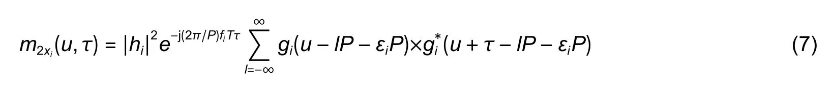
wherelPis the sampling time period of thelth symbol.
According to (7),the following expression can be proved

Equation (8) indicates thatm2xi(u,τ) is a periodic function,whose Fourier series can be expressed as

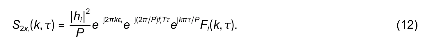
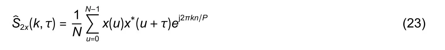
whereS2xi(k,τ) is also called as the cyclic auto-correlation function ofxi(u).
According to the Parseval’s theorem,we get

whereGi(f) is the Fourier transform ofgi(m).
Let

Then,(9) can be rewritten as
Becausex1(t),x2(t),andv(t) are mutually independent,the auto-correlation function of the multi-carrier mixed signal can be expressed as

Thus,the cyclic auto-correlation function ofx(u) can be written as
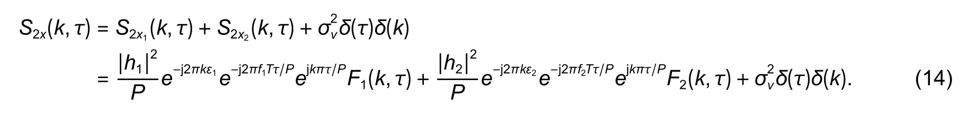
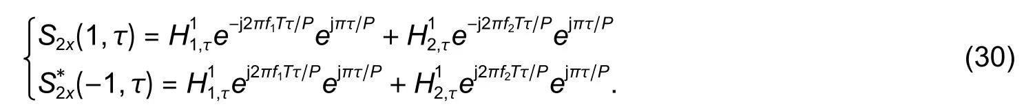
Whenk≠0 orτ≠0,(14) can be simplified as

Based on the cyclic auto-correlation function,we will discuss the timing estimation algorithms whenh1,h2,F1,andF2are known or not,respectively.
3.1.Method I
At the time,the parametersh1,h2,F1,andF2are assumed to be known at the receiver.S2x(k,τ) can be rewritten as

A=∣h1∣2F1(k,τ)/P B=∣h2∣2F2(k,τ)/P
where,,and
In (16),the real and imaginary parts can be expressed as
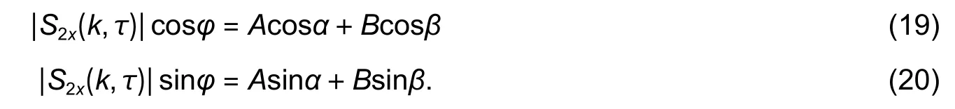
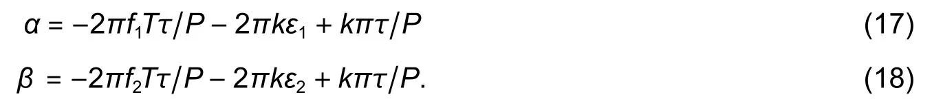
From the received data,S2x(k,) can be calculated similarly.Thus,∣S2x(k,τ)∣andφare considered to be known in (19) and (20).Becauseh1,h2,F1,andF2are the prior knowledge,the variablesAandBare also known at this time.Then there are only two unknown variables in (19) and (20),i.e.,αandβ.At this situation,αandβcan be directly obtained by solving (19) and (20).They are expressed as

In (21),because of the vague characteristics of the blind signal processing,there are two different solutions.The error of the solution can be eliminated by using auxiliary data.
From (17) and (18),it can be known that the time delayε1andε2of the multi-carrier mixed signal can be estimated by

when the variablesαandβare obtained.
Reviewing the above analyses,Method I can be summarized as:
1) Calculate the cycle auto-correlation functionof the multi-carrier mixed signal by
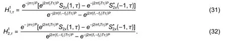
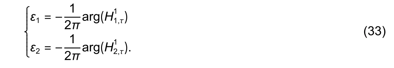
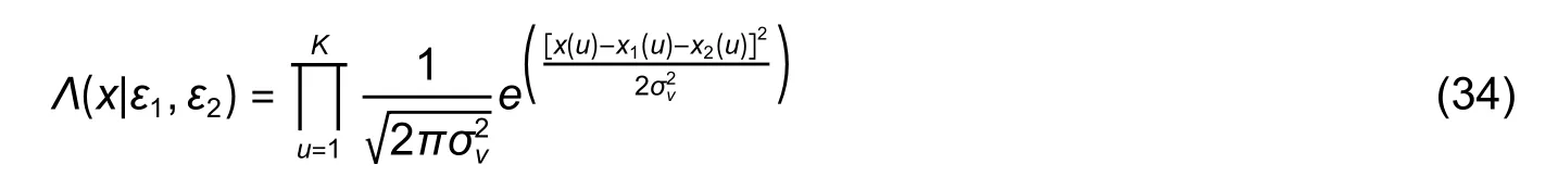
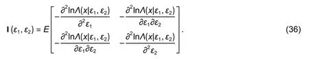
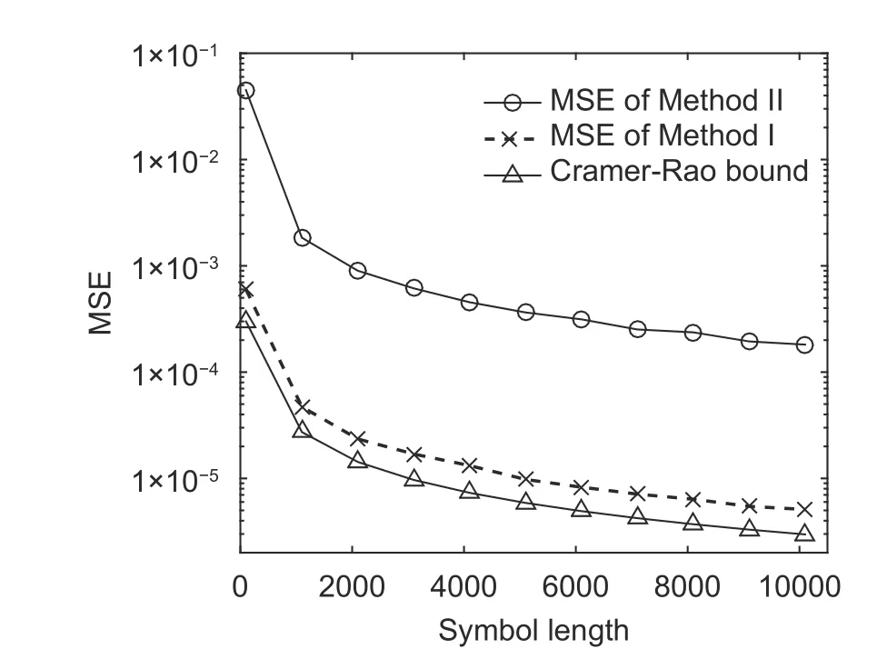
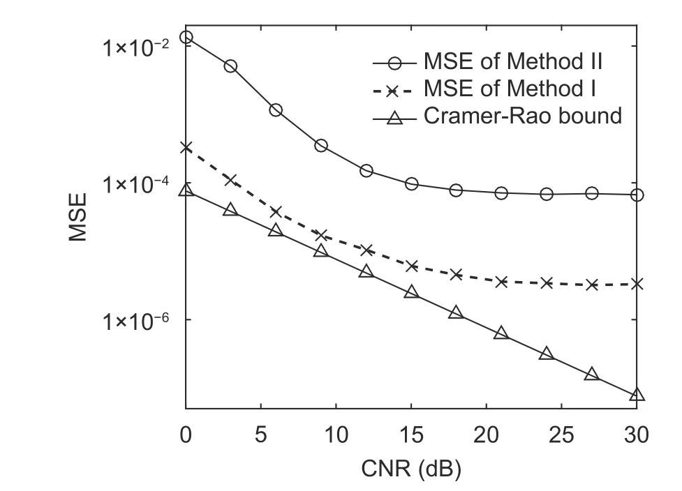
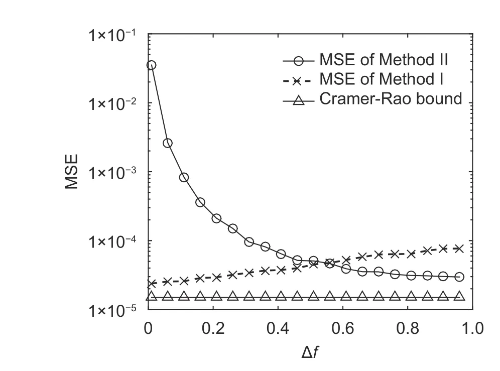
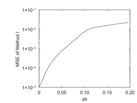
wherek=±1;0≤τ≤D,D 4) Letτ=τ+1.Ifτis less thanD,the process returns to 1),otherwise the process is terminated. In order to improve the precision,the mean value of the estimated results is considered as the final result,which is calculated by In practical applications,there are many scenarios where the parametersh1,h2,F1,andF2are unknown at the receiver.Method I is not suitable for this circumstance.In the following,we will approach another algorithm. Equation (15) can be rewritten as where Whenk=±1,we have In general,gi(t) is a raised cosine filter with a limited band,and it is a real-dual function.Thus,we have From (26),the following equation can be proved: Then,(27) can be rewritten as Equations (31) and (32) are effective if and only iff1is not equal tof2.In practical applications,the condition is usually satisfied.Then,the time delay,ε1andε2,can be acquired fromas follows From the above analyses,Method II can be summarized as: 3) Acquire the estimated time delayby (33). 4) Letτ=τ+1.Ifτis less thanD,the process returns to 1),otherwise the process is terminated. Similar to Method I,Method II also chooses the mean value of the estimated results as the final result. Compared with Method I,there are more unknown parameters in Method II,which essentially estimates the channel gain and the time delay at the same time.Thus,the performance of Method I is better than that of Method II,while the applicable range of Method II is more extensive. In this part,the Cramer-Rao bound of the timing estimation of the mixed OFDM signals is analyzed.The time delay is considered to be invariable in a short period.From (4),the likelihood function is given whereKis the length of the symbols. According to the Cramer-Rao inequality of the certain unknown parameter[3],[18],we have whereJi,iis the diagonal element in the matrix I−1,and I is the Fisher information matrix,which can be expressed as Becausex1(t),x2(t),andv(t) are mutually independent Thus,the Cramer-Rao bound can be expressed as In (40),the theoretical bound is closely related with the parameters,including the symbol lengthK,noise poweroversample rateP,and channel gainhi.With the increase ofK,P,orhi,the Cramer-Rao bound will become smaller,vice versa. In this paper,the Cramer-Rao bound is used to evaluate the performance of the proposed algorithms.In this section,two independent OFDM signals are produced,whose signal parameters are the same except the carrier frequency.The number of the subcarriers is 32,the symbol rateRbis 512,and the sub-carrier signals are QPSK signals.The oversampling ratioPis 8.The raised cosine filter with the roll-off factor of 0.3 is used as the pulse response.Without losing generality,the OFDM signals do not contain the cyclic prefix,the time delays are 0.3Tand 0.5T,respectively. The mean square error (MSE) of the estimated time delay is defined as When the number of OFDM symbols is equal to 2000,MSE of the estimated time delay with different carrier-to-noise ratios (CNRs) is shown in Fig.1. In Fig.1,MSE becomes smaller with the increase of CNR,when CNR is less than 18 dB.However when CNR is bigger than 18 dB,MSE is almost stable.MSE of Method I is obviously smaller than that of Method II. For the proposed algorithms,MSE mainly comes from the noise and statistical error.When CNR is smaller,the leading impact is from the noise.At this situation,MSE is improved with the increase of CNR.When CNR is big enough,MSE is mainly affected by the statistical error,which is closely related with the symbol length.In this experiment,the noise is the only variable,so MSE becomes better and better in the low noise situation,and it keeps steady in high CNR. When CNR is 10 dB,MSE of the estimated time delay with different symbol lengthsKis shown in Fig.2. In Fig.2,MSE becomes smaller when the symbol length increases.Compared with the result of Method II,MSE of Method I is smaller,which is close to the Cramer-Rao bound. Fig.2.MSE versus symbol length K. Similar to Experiment 1,MSE fluctuates with the change of the statistical error when CNR is given,which is determined by the symbol length. Let Fig.1.MSE versus CNR. wherefiis the carrier frequency of theith OFDM signal and Δfis the normalized frequency interval. When the symbol number is 2000 and CNR is 10 dB,the simulation results for different normalized frequency intervals is shown in Fig.3. In Fig.3,MSE of Method II is continuously improved with the increase of the normalized frequency interval.The performance change of Method I is very small. In Method II,the denominator of (31) and (32) can be expressed as In (43),the modulus of Mid is proportional to s in(2πΔfTτ/P).Thus,MSE becomes smaller with the increase of ΔfwhenPis larger than 4.This means that the estimation performance of Method II becomes better with the increase of the frequency interval when the oversample ratePis larger than 4. In Method I,the estimated time delay is only related with the carrier frequency,while it is not connected with the frequency interval.Thus,the performance of Method І is almost not affected when the frequency interval changes. Let wherefiis the real carrier frequency,is the estimated carrier frequency,and dfis the normalized frequency error. When CNR is 15 dB and the symbol length is 2000,the simulation results of Method I at different normalized frequency errors are shown in Fig.4. Fig.3.MSE versus frequency interval Δf. Fig.4.MSE versus frequency error df for Method I. In Fig.4,MSE of Method I becomes larger with the increase of dfwhenτis not equal to 0.Whenτis equal to 0,MSE keeps stable. Reviewing (22),it can be rewritten as whereustands forαorβ. In (45),the estimated time delayεiis related with the carrier frequencyfiif and only ifτis not equal to 0,which is consistent with the simulation result.In practice,the frequency error is inevitable,so the value ofτis usually equal to zero to eliminate the effect of the frequency error. When CNR is 15 dB and the symbol length is 2000,the simulation results of Method II at different frequency errors are shown in Fig.5. In Fig.5,MSE of Method II becomes larger with the increase of the frequency error,and the two curves are almost overlapped. Reviewing Method II,it is effective whenτis not equal to 0.Thus,the influence of the frequency error is unavoidable.To ensure the demodulation performance,the frequency error is required to be less than 2%. Let wherehiis the real amplification,is the estimated amplification,and dhstands for the amplification error. In Method II,the amplification is unknown at the receiver,so it is uncorrelated with the amplification error. When CNR is 15 dB and the symbol length is 2000,the simulation results of Method I at different amplification errors dhare shown in Fig.6. Fig.5.MSE versus frequency error df in Method II. Fig.6.MSE versus amplification error dh. In Fig.6,MSE become larger when the amplification error increases.To ensure the demodulation performance,the amplification error should be less than 8%. According to the simulation results,we can conclude that the performance of the proposed algorithms is closely related with CNR and the symbol length.Besides,the performance of Method I will be affected by the amplification precision,while the performance of Method II is related with the frequency interval and frequency precision. In this paper,two timing estimation algorithms are proposed for the mixed OFDM signal.Method I is applied when the channel gain and filter have been known at the receiver.When the prior information is unknown,Method II is used to estimate the time delay and channel gain.Method I has better performance,while Method II has a more extensive application range.The performance of the proposed algorithms is closely related with CNR,the symbol length,frequency precision,amplification precision,and frequency interval.In the following research,our further study will be focused on how to separate the mixed OFDM signal. This work was supported by National Key Laboratory of Science and Technology on Blind Signal Processing,and the work is supervised by the Prof.Zhong-Liang Zhu.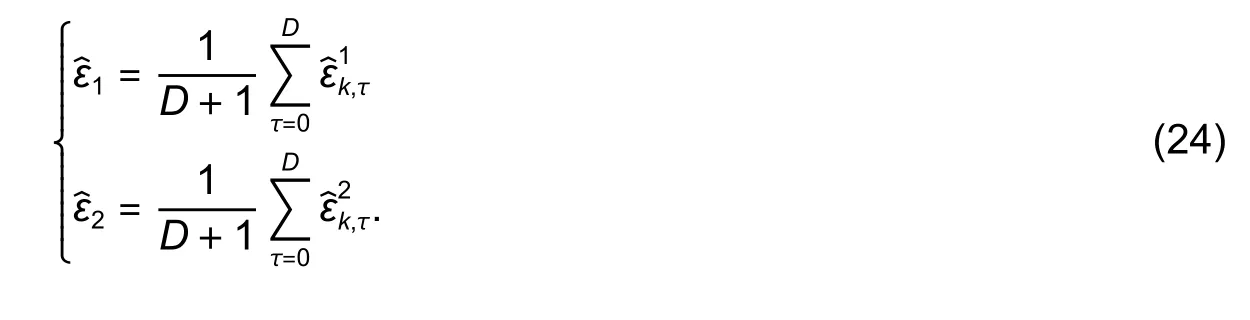
3.2.Method II


3.3.Cramer-Rao Bound

4.Performance Analysis and Simulation

4.1.Experiment 1
4.2.Experiment 2
4.3.Experiment 3


4.4.Experiment 4


4.5.Experiment 5

5.Conclusions
Acknowledgment
 Journal of Electronic Science and Technology2020年3期
- Journal of Electronic Science and Technology的其它文章
- Call for Papers Special Section on Energy and Environmental Materials
- Numerical Analysis of Artificial Electron Heating Effects on Polar Mesospheric Winter Echoes
- Systematic Synthesis of Compressive VDTA-Based T-T Filter with Orthogonal Control of fo and Q
- MUSIC-Based Pilot Decontamination and Channel Estimation in Multiuser Massive MIMO System
- High Capacity Data Rate System:Review of Visible Light Communications Technology
- Light-Weight Selective Image Encryption for Privacy Preservation