A 3D CNN Molecular Clump Verification Method for MWISP Project∗

ZHOU Piao LUO Xiao-yu ZHENG Sheng JIANG Zhi-bo ZENG Shu-guang

(1 College of Science, China Three Gorges University, Yichang 443002)(2 Center of Astronomy and Space Science Research, China Three Gorges University,Yichang 443002)(3 Purple Mountain Observatory, Chinese Academy of Sciences, Nanjing 210023)

ABSTRACT Molecular clumps are the birth place of stars. A census of molecular clumps and comprehensive studying of their properties will help us to understand the star formation process and the evolution of the Galaxy and the Universe. As the MWISP (Milky Way Imaging Scroll Painting)project going to be completed, such a kind of studies become to be practicably feasible. With the large amount of data at hand, an algorithm that automatically identifies and verifies molecular clumps is urgently in need.For the widely used methods for the three-dimensional molecular line data,including GaussClumps, ClumpFind, FellWalker, and Reinhold, one has to input a number of parameters to control their performances, which need to be repeatedly optimized and visually inspected, and then to obtain a satisfactory result. Therefore it is a human-power and time consuming task to identify and verify clumps for large-scale survey data. To overcome the limitations of the traditional clump detection algorithms, artificial intelligence(AI) would be a good solution. Here we propose a 3D CNN (Convolutional Neural Network) method, which can perform the task automatically. The whole process is divided into two steps, i.e., identification and verification.First we use traditional method (ClumpFind) with low threshold to identify candidates. The verification is done by trained 3D CNN models. We have done a series of experiments using artificial data. The results suggest that our method is advantageous over the four traditional methods. Application of the method to the real MWISP data demonstrates that the performance of the 3D CNN method is also satisfactory.

Key words stars: formation, ISM: clouds, techniques: image processing

1 Introduction

The structures that can be detected by CO in interstellar medium are collectively referred to as molecular clouds, and the dense molecular cloud structure inside which stars may form is called clumps[1–2]. It has become the consensus of astronomers that stars originate in molecular cloud clumps. So far, the processes that convert molecular gas into stars are still unclear[3]. The MWISP (Milky Way Imaging Scroll Painting) project is dedicated to the large-scale survey of12CO(J=1-0),13CO(J=1-0), and C18O(J=1-0)lines,along the northern Galactic Plane. The project is implemented with the Purple Mountain Observatory Delingha(PMODLH-13.7 m)telescope[4−5]. The data product can be used to identify molecular clumps and analyze their properties, etc.,thus provide a promising opportunity to study the earliest stages of star formation.

For a large-scale project, such as the MWISP survey, one needs full-automatic methods to analyse the data, especially in detecting clumps in various environments.While a number of methods have been developed for identifying clumps, they are actually not intelligent enough to do the work automatically. The typical algorithms include GaussClumps, ClumpFind, FellWalker, Reinhold, etc.

The GaussClumps algorithm[6], performs least-square fits with Gaussian function to the brightest spot in the data. There are 19 parameters in GaussClumps algorithm, three of which are key parameters to control the detection background threshold(THRESHOLD) and the minimum size of the clumps (FWHMBEAM, VELORES).The ClumpFind algorithm[7]contours the data cube above a certain level, starting from the brightest peak in the data. This technique was “motivated by how the eye decomposes the maps into clumps” and it “mimics what an infinitely patient observer would do”. This method ignores the backgrounds in which clumps are observed.There are 11 parameters in the ClumpFind algorithm, two of which are the key parameters to control the detection background threshold (TLOW) and contour interval(DELTAT).The FellWalker algorithm,proposed by Berry[8],works in a similar way to a mountaineering process,which starts from some of the relatively low-intensity locations, searching along the direction of the largest gradient until a common peak location is found. Finally, all pixel points in all paths converging on the same maximum value are grouped into a clump. There are 11 parameters in FellWalker algorithm,three of which are the key parameters to control the minimum strength of clumps(MINHEIGHT)and to distinguish adjacent clumps (MINDIP, MAXJUMP). The Reinhold algorithm[9]is opposite to FellWalker, looking down from a relatively high-intensity position below a certain threshold as a boundary.

These existing algorithms have many parameters to control their performances for specific project, which needs to be optimised in a number of iterations. Although they can achieve satisfactory performances for specific data after repeated optimization,the process is complex, time-consuming, and uncertain for different analysers, and the identified clumps still need to be manually verified. Now,with the scheduled progress of the MWISP project, molecular cloud data is rapidly accumulating, and it is impossible to be manually processed and verified. One cannot expect high levels of detection completeness and accuracy in realistic MWISP project condition from such methods without huge human-power. To overcome the limitations of existing molecular clump detection algorithms,a fully automated clump detection method,which does not require frequent human interaction, needs to be developed urgently. A promising candidate would be the rapidly advancing artificial intelligent field called deep learning, which is a highly scalable machine learning technique that can learn directly from raw data,without any manual feature extraction.

In recent years, the most concerned topics in the field of deep learning is the Convolutional Neural Network (CNN). Since 2012, AlexNet[10]has been proposed as a CNN and achieved the best performance of ImageNet database[11]. The deep learning algorithm represented by CNN is widely used in image recognition[12−14], target detection[14−16], and image segmentation[17]. CNN has also been successfully applied in recognition and classification of astronomical images. Petrillo et al.[18]trained CNN with a self-made image to carry out gravitational lens candidate recognition. George et al.[19]injected the generated signal into the LIGO (Laser Interferometer Gravitationalwave Observatory) data to train CNN, and used the trained CNN to detect the gravitational wave. Different from the above examples, the products of MWISP are three dimensional data with two dimensions as position, and one as velocity. The scale and shape of molecular cloud clumps themselves are highly variable. To automatically identify and verify the molecular clumps from the position-velocity data cube of the MWISP project, we propose a combination method, in which a CNN model, Voxnet[20]is applied to the verification process. For comparison we also try another CNN model(i.e. Multi-view CNN[21]). The structure of this paper is arranged as follows. In section 2, we introduce the method. The analysis and results of this method, and comparison to the traditional algorithms are discussed in the third section; In section 4, we give the conclusion.

2 Method

2.1 Detection process

The whole process of the detection is shown in Fig.1. Firstly we use ClumpFind to identify clump candidates within the original 3D data. The second step is to verify the candidates as positive or negative. Finally the catalog of the clumps is exported for future scientific studies.

Fig. 1 A schematic view of the molecular clump detection process

The second step, i.e., verification is the crucial one of this work. The trained CNN models are used to verify candidates, the whole process of the verification includes following steps:

(1) Making samples;

(2) Training the CNN model;

(3) Labeling the clump candidates as positive or negative.

2.2 CNN model

There are two types of classification methods to deal with 3D data. One is work on raw 3D data directly (e.g., polygon mesh, discretization based on “voxel”, point cloud, etc.), and the typical models are 3D ShapeNets and Voxnet. Among them, 3D ShapeNets is more suitable for detecting the surface shape of 3D objects. Voxnet uses voxel grid to describe point cloud data in voxel grid. The voxel grid data are similar to MWISP data, so we chose Voxnet as the classification model. The other is to use several 2D projections to describe 3D objects, in this work, a 3D sample is replaced by three integral images in different directions. We designed a CNN model (i.e. Multiview CNN),and compare with the other 3D CNN model(i.e. Voxnet)to see which one performs better.

The Voxnet model has two convolutional layers with a convolution kernel size of 5 and 3, and two fully connected layers with 128 and 10 neurons, respectively. The entire process is activated using Relu (Rectifiled Linear unit). We used 32 kernels for all the convolutions and 2 strides for the only (max) pooling layers. In this work, as illustrated in Fig.2, we set the number of neurons in the last layer to 2 for the positive and negative classification of clumps.

The Multi-view CNN model consists of three independent AlexNets[10], each has five convolutional layers with a convolution kernel size of 11×11×3,5×5×48,3×3×256,3×3, and 3×3, and three fully connected layers with 4096, 4096, and 1000 neurons,respectively. As is shown in Fig.3, in the input layer, the input data were projected to the X-axis, Y-axis, and Z-axis respectively to obtain three gray images of 227×227.Each gray image was copied into the RGB channel, finally obtaining three samples of 227×227×3. We train AlexNet1 with the samples obtained from theX-axis integral,AlexNet2 with the samples obtained from theY-axis integral, and AlexNet3 with the samples obtained from theZ-axis integral. In this work, we set the number of neurons in the last layer of AlexNet to 2 for the positive and negative classification of clumps.Finally, in the testing process the classification results are output by voting.

Fig. 2 The VoxNet Architecture. C(x,y,z) indicates that the convolutional layer has x filters of size y and at stride z, P(d) indicates pooling with an area d, and F(k) indicates fully connected layer with k outputs.

Fig. 3 The Multi-view CNN architecture

3 Experiments

3.1 Experimental data set

A successful verification process relies on stable trained CNN model,and the model relies on the distinction of the training dataset. Our first step is to make artificial samples. The generated dataset can be used to directly quantify the performance of the method, and easily compare with other four traditional methods.

Our simulated clumps were obtained by Cupid.makeclumps in the Starlink software1Starlink software is freely available astronomical data reduction and analysis software, available from http://starlink.jach.hawaii.edu..Each clump has a Gaussian profile with FWHMs (Full Width at Half Maximums) randomly ranging between 4–14 pixels in the first two dimensions(position)and 4–12 pixels in the third dimension (velocity). The peak values are distributed uniformly between 10 and 30.

In this experiment we always inject 100 simulated clumps of different peaks into the data cubes. We make a large amount of cubes with Gaussian noises ranging between 1–20, indicating the signal-to-noise ratio of sample between 0.5–30. To simulate the real data of different source densities, 3 kinds of cubes are generated with sizes of 100×100×100 (hereafter Cube1), 150×150×150 (Cube2), 200×200×200 (Cube3) voxels.

The next step is to make samples. For generated data cubes, we use ClumpFind to identify candidates with default parameters (DELTAT = 2 RMS, TLOW = 2 RMS,RMS is the root mean square error). The output of ClumpFind is classified into two groups. Those injected clumps are put into the positive group, while the others are put into the negative group. Then we extract small cubes centered on the members of the two groups. The size of the small cubes is fixed to 15×15×19 voxels. After the normalization of each small cubes, the samples are ready for the training and testing.

For the training process, the sample set is composed of more than 10000 positive and negative samples, which are divided into the training set and the validation set according to the ratio of 4:1.

For the testing process,we generated 15 new cubes in different sizes and source densities in the same manner to training set. Again,we obtain candidates using ClumpFind and extract small cubes. The small cubes corresponding to candidates are input into the CNN models, which flag out the candidates as positive or negative. The whole program to flag the candidates as positive or negative is referred to as a classifier. Finally, scoring the performance for each algorithm. For comparison, the four traditional methods, i.e., ClumpFind, GaussClumps, FellWalker, and Rainhold, are also tested for these new cubes. The parameters for the four methods are set to default supplied by the Cupid.findclumps in the Starlink software.

3.2 Experimental parameter setting

It should be noted that the two models have different requirements on the size of input data. In the operation of input layer, the input data are adjusted to the size required by the model through nearest neighbor interpolation algorithm and “same padding”.

About the training process, the ReLu is used as the activation function for the two models to make a nonlinear mapping for the output results of the convolutional layer, which enhances the expression ability of the data coefficient and the nonlinear expression ability of the CNN model, so that the model can better adapt to complex problems, at the same time choose Adam (Adaptive moment estimation) and SGDM(Stochastic Gradient Descent-Momentum) respectively as these two learning rules of the model to optimize the training process. We describe the training paramenters of the Voxnet model and Multi-view CNN model in Table 1. The loss values of both the training set and the validation (train_loss, val_loss), and the accuracy of both the training set and the validation(train_acc,val_acc)are comprehensively used to evaluate the effectiveness of model in the training process.

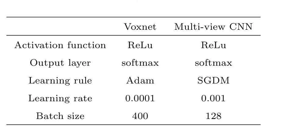
Table 1 Hyper parameters of two CNN models. We have used the same set of hyper parameters for both the simulated and MWISP data (M16) datasets.

3.3 Scoring the performance

According to the input and output, four statistics are obtained. They are: True-Positive (TP), True-Negative (TN), False-Positive (FP), and False-Negative (FN).

•TP: Number of samples belonging to the TRUE class, which are correctly labeled by the classifier as positive;

•TN:Number of samples belonging to the FALSE class,which are correctly labeled by the classifier as negative;

•FP: Number of samples belonging to the FALSE class, which are incorrectly labeled by the classifier as positive;

•FN:Number of samples belonging to the TRUE class,which are incorrectly labeled by the classifier as negative.

An ideal classifier requires both high recall rate (r) and detection precision (p),which are defined as:

where thervalue ranges between 0 and 1, and 1 implies that all candidates in the TRUE class are labeled as positive. This parameter is prominent, when misclassifying a TRUE sample has a higher cost than misclassifying a FALSE sample. Thepis a ratio of TRUE class labeled correctly to the total number of incidence, which are labeled as positive (irrespective of whether they are true positives or not).

In order to combine the two parameters into a single score, we defineF1, which is the harmonic mean ofpandr, i.e.

where the definition ofF1indicates thatrandpare of the same weight.F1ranges between 0 and 1, which can signify the performance of different methods. The value 1 indicates a perfect performance while 0 indicates poor.

3.4 The results for the simulated data

In Section 3.2, after the training set have been adjusted to the required input size of the model,Multi-view CNN and Voxnet are trained respectively,and the recognition accuracy and loss change curve of the verification set are shown in Figs.4 and 5 respectively. The abscissas in Figs.4 and 5 are the number of network iteration steps. The left vertical axis represents the loss value of training set and validation set; the right vertical axis represents the accuracy of recognition.

Since the Multi-view CNN in this paper is composed of three independent AlexNets,three different loss and accuracy curves will be output during the training process. As shown in left panels of Fig.4(a)(b)(c), the loss values of both the training set and the validation set gradually decrease to a low level after 100 epochs, and the changes tend to be flat. The panels on the right of Fig.4(a)(b)(c) show that in the training process,the accuracy curve of the validation set of the three AlexNet models all began to flatten after 150 epochs. The final accuracy of AlexNet1 and AlexNet2 reached 0.85, and the final accuracy of AlexNet3 reached 0.76. As the output results of Multi-view CNN model were voted by AlexNet1, Alexnet2, and Alexnet3, the accuracy of this model could be predicted to be higher than that of the single AlexNet model. Voxnet uses 3D data for the experiment, there is less information loss. Compared with the loss and accuracy curve of Multi-view CNN, Fig.5 shows the accuracy curve of Voxnet model converged faster and had a higher accuracy, reaching the highest level (0.92) around the 75th round.

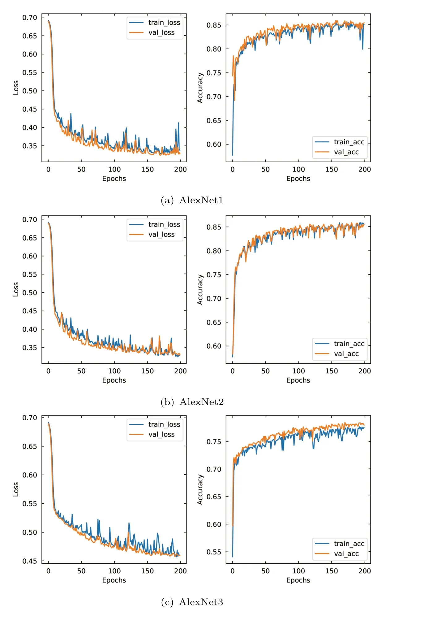
Fig. 4 Classification accuracy and loss curve of Multi-view CNN model based on simulation samples,which is composed of three independent AlexNet models.

Fig. 5 Voxnet CNN model classification accuracy and loss curve based on simulation samples.

In order to inspect the effectiveness and reliability of the models, we use artificial samples of different densities to test trained Voxnet model and Multi-view CNN model.It is found that adjusting the input sample size has little effect on the experimental results of the two models. Table 2 shows the results of our tests for Voxnet, Multi-view CNN, and four traditional methods. As expected, 3D CNN methods, especially the Voxnet method, performs stabler than the others. TheF1values of the Voxnet method range between 0.78 and 0.89 in three different environments, with an average of 0.84.This is virtually better than all other methods. FellWalker algorithm, which performs best after testing by Li et al.[22], gives a high overallvalue. However, this is because that it performs very well in the sparsely populated environments. In dense regions,thervalue is not satisfactory.

Table 2 Detection results by different methods.is defined as the mean of F1

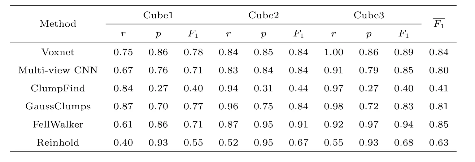
Table 2 Detection results by different methods.is defined as the mean of F1

Method Cube1 Cube2 Cube3 F1 r p F1 r p F1 r p F1 Voxnet 0.75 0.86 0.78 0.84 0.85 0.84 1.00 0.86 0.89 0.84 Multi-view CNN 0.67 0.76 0.71 0.83 0.84 0.84 0.91 0.79 0.85 0.80 ClumpFind 0.84 0.27 0.40 0.94 0.31 0.44 0.97 0.27 0.40 0.41 GaussClumps 0.87 0.70 0.77 0.96 0.75 0.84 0.98 0.72 0.83 0.81 FellWalker 0.61 0.86 0.71 0.87 0.95 0.91 0.92 0.97 0.94 0.85 Reinhold 0.40 0.93 0.55 0.52 0.95 0.67 0.55 0.93 0.68 0.63

Therefore, it is not recommended for clump-extraction in dense regions, which is frequently the case of13CO clumps. On the other hand,as the accumulation of training set in the real work, the 3D CNN method is expected to perform better and better.We note however, the performance of the four traditional methods can be improved by deliberate adjustment of input parameters, but this is only applicable in studying individual fields – it is not reasonable to utilize for the study for large areas in the era of big-data.

3.5 Testing for real data

In order to check if the Voxnet performs satisfactorily as well towards real data,we use the M16 region as a show-case. The13CO data from the MWISP project are adopted here. With the GaussClumps parameters setting (RMS = 0.3 K, FWHM BEAM = 52.0′′, FWHM START = 1.5, VELO RES = 0.167 km·s−1, VELO START =60.0,THRESHOLD=4.0 K),approximately 500 clumps have been verified by Song[23].By visual inspection, we believe that 432 of them are real clumps. ClumpFind with lower threshold can produce a large number of false detections, we regard 1926 false detections as negative samples. It is not enough to train and test the CNN model.Using data augmentation such as translation, zooming, and rotation, we finally obtain 9072 positive samples and 9276 negative samples. Both positive and negative samples are randomly divided into two groups, in which 85% are used for model training and 15% for testing, respectively.

In Fig.6,we present the samples before augmentation,which used to train Voxnet.“∗” represents the position of the positive samples, and “+” represents the position of the negative samples. The results of verification by Voxnet algorithm are shown in Fig.7. “∗” and “+” represent the positive and negative test samples, respectively.Circles represent those being properly classified (i.e., true clumps labeled as positive and false detection labeled as negative). From the figure,we can see that all the positive samples have been correctly verified by Voxnet. Only a small portion of negative samples were misclassified. The values ofr,p, andF1are calculated to be 1, 0.89, and 0.94,respectively, indicating that Voxnet is promising in working on real data.

Fig.8 shows the curve of loss and accuracy during training. The left panel shows the variation curve of the loss function during training, and it can be seen that the loss gradually converges to a smaller value (less than 0.05). The right panel shows the variation curve of the accuracy function during training, and the accuracy gradually converges to a larger value (greater than 0.98). Overfitting may occur after the 30th epoch, so we take the model at the 20th epoch as the best model to conduct the above test experiment. The testing results suggest that Voxnet is also suitable for MWISP real data sets.

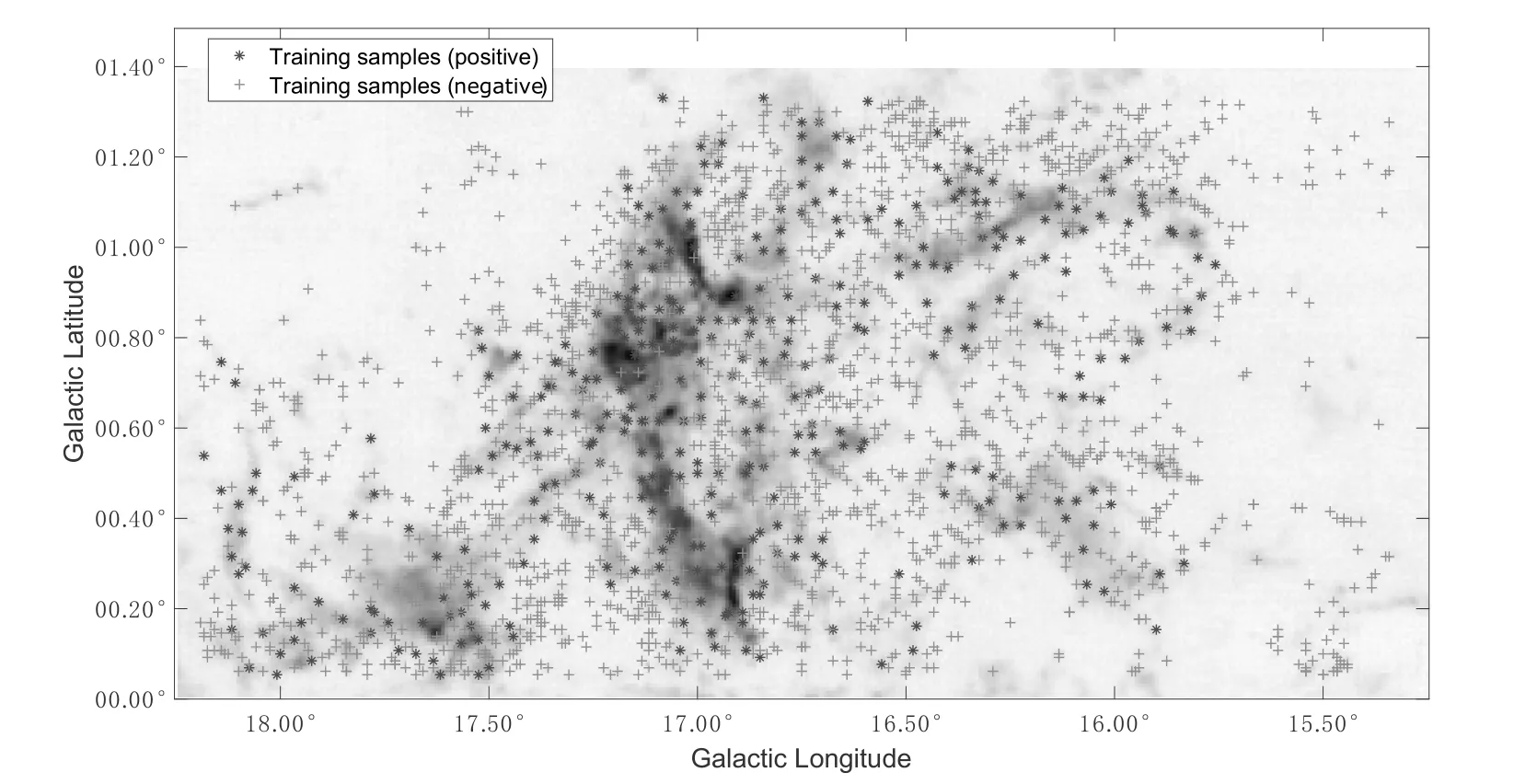
Fig. 6 Data samples used to train Voxnet, and the background image is the integrated intensity of 13CO in M16. “∗” represents the position of the positive samples, and “+” represents the position of the negative samples.

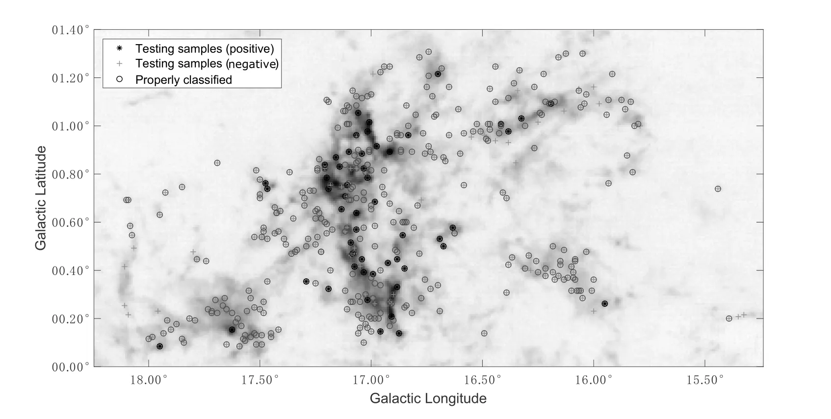
Fig. 7 Voxnet verification result, and the background image is the integrated intensity of 13CO in M16.“∗” and “+” represent the positive and negative test samples, respectively. Circles represent those being properly classified (i.e., true clumps labeled as positive and false detection labeled as negative).

Since the morphology of clumps is far more complicated in real data than in artificial data, more experiments are necessary to prove the solidity of the method. At the beginning of the process,large amount of human-power is needed in visual inspection of real clumps. As the work proceeds on,we believe that less and less human inspection is necessary in building up training set,and that we can achieve a concrete model towards automatical identifying and verifying molecular clumps with little human interaction.

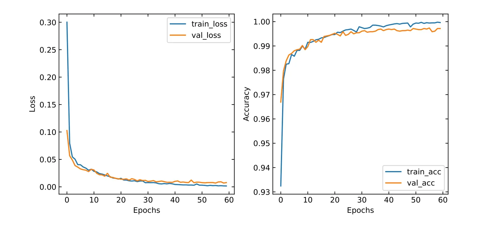
Fig. 8 Classification loss and accuracy during training process of Voxnet

4 Conclusion

We propose here a 3D CNN method, to identify and verify molecular clumps automatically for the MWISP data. The whole process of the method has two steps:identification and verification. The candidates are firstly obtained by the classical algorithm ClumpFind with very low threshold and then verified with 3D CNN models.The method has the advantage over the existing molecular clump detection algorithms in that it does not need frequent interaction between machine and human in optimizing parameters. The experimental results on simulated data demonstrate that the performance of the 3D CNN method is better than those of the traditional methods in different kinds of environments. Applying this method to the real M16 suggests that it works satisfactorily as well. The Voxnet is a promising tool in automatically detecting molecular clumps with little human interactions for the large amount of 3D data in the big data era.