
ARTIAL REGULARITY FOR STATIONARY NAVIER-STOKES SYSTEMS BY THE METHOD OF A-HARMONIC APPROXIMATION*
2020-08-03 13:10:54YichenDAI戴祎琛
Yichen DAI (戴祎琛)
School of Mathematical Sciences, Xiamen University, Fujian 361005, China
E-mail: yichendai0613@163.com
Zhong TAN (谭忠)
School of Mathematical Science and Fujian Provincial Key Laboratory on Mathematical Modeling and High Performance Scientific Computing, Xiamen University, Fujian 361005, China
E-mail: tan85@xmu.edu.cn
Abstract In this article, we prove a regularity result for weak solutions away from singular set of stationary Navier-Stokes systems with subquadratic growth under controllable growth condition. The proof is based on the A-harmonic approximation technique. In this article,we extend the result of Shuhong Chen and Zhong Tan [7] and Giaquinta and Modica [18] to the stationary Navier-Stokes system with subquadratic growth.
Key words Stationary Navier-Stokes systems; controllable growth condition; partial regu-larity; A-harmonic approximation
1 Introduction and Statement of the Result
Throughout this article, on a domain, where is a bounded with Lipschitz boundary in Rnwith dimension n ≥ 2, we consider weak solutions u:Ω→RNof stationary Navier-Stokes systems of the type
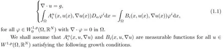
1.1 Assumptions on the structure functions
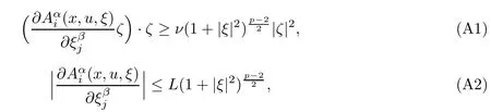
for all x ∈Ω, u ∈RN, and ξ, ζ ∈RNn, where ν, L>0 are given constants.
There exist β ∈(0,1) and K :[0,∞)−→[1,∞) monotone nondecreasing such that

Furthermore,we assume that there is a function ω :[0,∞)×[0,∞)−→[0,∞)with ω(t,0)=0 for all t such that t →ω(t,s) is monotone nondecreasing for fixed s, where sω(t,s) is concave and monotone nondecreasing for fixed t, and such that
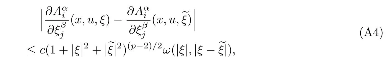
for all x ∈Ω, u ∈RN, and ξ,∈RNn.
1.2 Assumptions on the inhomogeneity Bi
For the inhomogeneity Bi, we assume that Bisatisfies the controllable growth condition

for all x ∈Ω, u ∈RN, and Du ∈RNn, where
Moreover, because of the growth assumptions above, it is easily seen that the classical Navier-Stokes system

in its weak formulation is included in (1.1) provided n ≤4.
Let us consider the Helmholtz-Weyl decomposition of the space Lp. Refer to the study of the relevant properties of these spaces by [17]:
Set
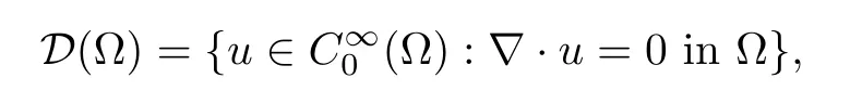
for p ∈[1,∞). We denote by Hp(Ω) the completion of D in the norm of Lpand put

Let ω be either a bounded or an exterior C2-smooth domain or a half space in Rn, n ≥2.
Then, Gp(ω) and Hp(ω) are orthogonal subspaces in Lp(ω). Moreover,

where ⊕denotes direct sum operation.
Furthermore,the validity of decomposition(1.2)implies the existence of a unique projection operator
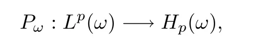
that is, of a linear, bounded, idempotent (= Pω) operator having Hp(ω) as its range and Gp(ω) as its null space.
As a result, we obtain, for all ϕ ∈W1,p0 (ω,RN),

The point of the technique of harmonic approximation is to show that a function is‘approximately-harmonic’. That is, a function g, for which
Ω Dg·Dϕdx is sufficiently small for any test function ϕ, lies L2-close to some harmonic function. The harmonic approximation lemma can be found in Simon’s proof[24]. Allad[2]and de Giorgi[11]developed the regularity theory of minimal surfaces (see [11]). Until now, the technique of harmonic approximation was developed further and adapted to various settings in the regularity theory (see [16]), for a survey on the numerous applications of harmonic type approximation lemmas. The harmonic approximation method allows the author to simplify the original ε-regularity theorem(see[25])because of Schoen-Uhlenbeck (see [26]).
In this article, we extend the result of Shuhong Chen and Zhong Tan [7] and Giaquinta and Modica [18] to the stationary Navier-Stokes system with subquadratic growth. However,Shuhong Chen and Zhong Tan [7] has proven the partial regularity under the controllable condition (B1) with polynomial growth rate p = 2. This controllable growth condition has not been used widely, even in the parabolic systems system (see [6, 10]. In this article, we fill this gap in the theory and prove the partial regularity with subquadratic growth under the controllable growth condition (B1).
Our work is organized as follows. First of all, we collect some preliminary material forms in Section 2, which will be useful in our proof. The first step of our proof is to establish a Caccioppoli type inequality in Section 3. Next, we derive decay estimate in Section 5,which characterizes the singular set, by using the A-harmonic approximation lemma stated in Section 2.
Next, we will state our main result as follows.
Theorem 1.1We assume that u ∈W1,p(Ω,RN) with ∇·u = g is a weak solution of systems (1.1) under the conditions (A1) to (A4), the controllable growth condition (B1), and g ∈L2(Ω).
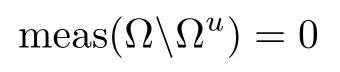
Then, there exists an open subset Ωu⊂Ω with

We point out that the Hölder exponent β of the gradient of the solution is the optimal one so that no higher regularity of the solution can be expected.
Moreover, we have the following characterization of the singular set.
Proposition 1.2In the situation of the preceding theorem, the singular set satisfies,moreover,
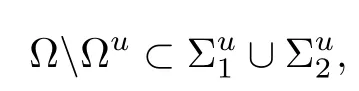
where
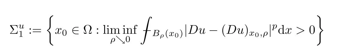
and
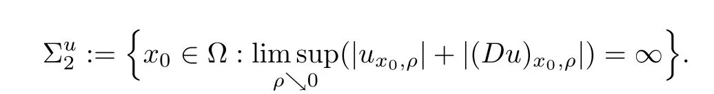
In the case of a structure function A(x,u,ξ) ≡A(x,ξ) that does not depend on u, the above statement remains true if we replace the setby

Furthermore, we have
and

2 Preliminary Material
2.1 The function V and W
We define

for all A ∈Rk, where k ∈N, which immediately yields

Then, we state some standard inequalities for later reference [1, 5].
Lemma 2.1For any 1 < p < 2, A,B ∈Rk, and V as defined above, we have the followings:
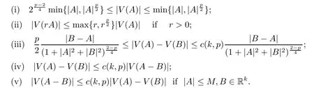
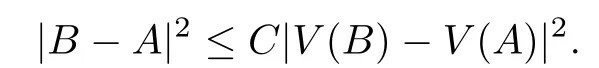
Immediately, we draw a conclusion that for |B −A|≤1,
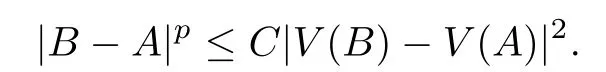
For |B −A|>1, we have
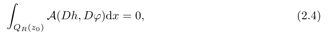
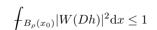
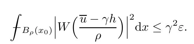
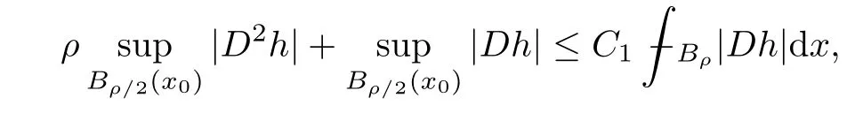
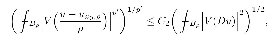
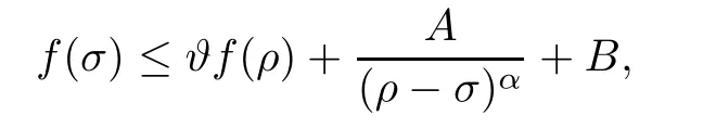
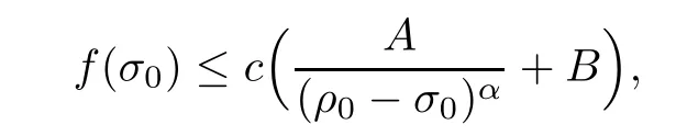
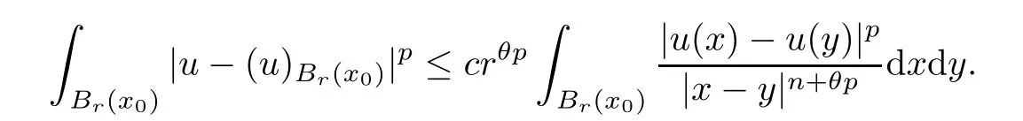
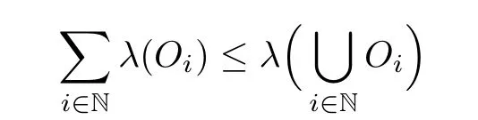
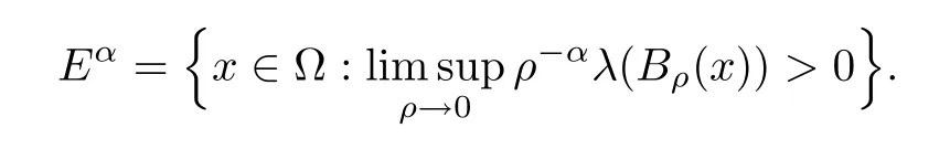
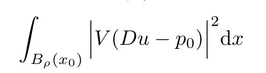
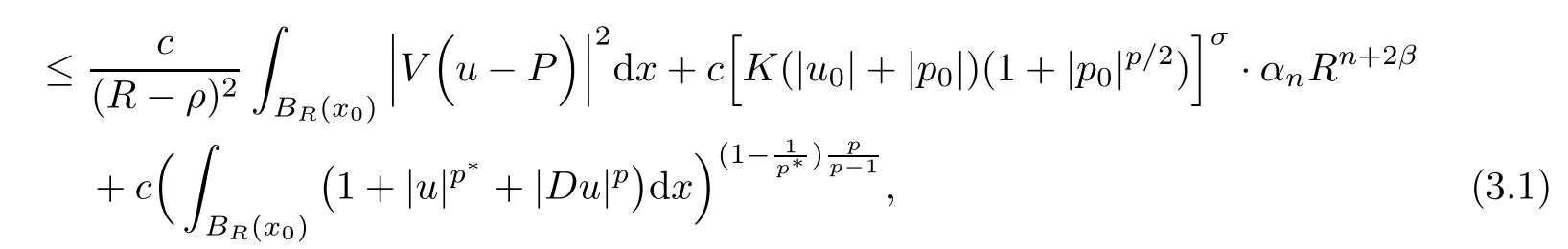
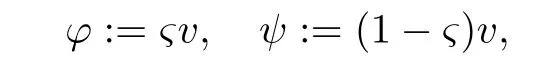
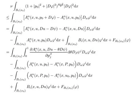
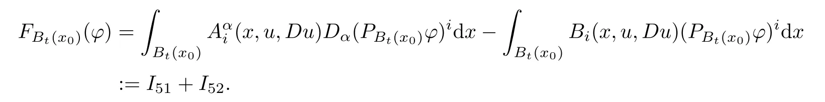
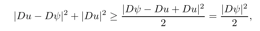
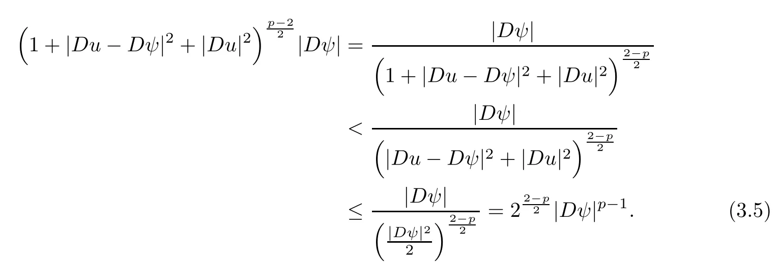
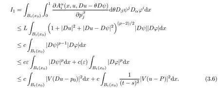
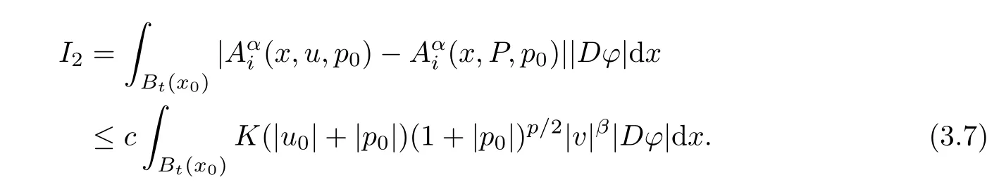
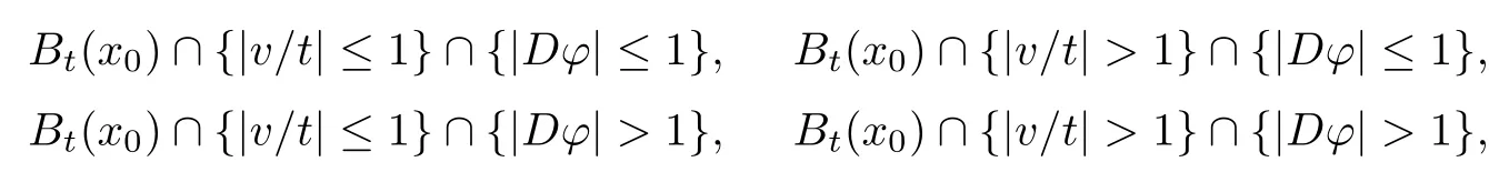
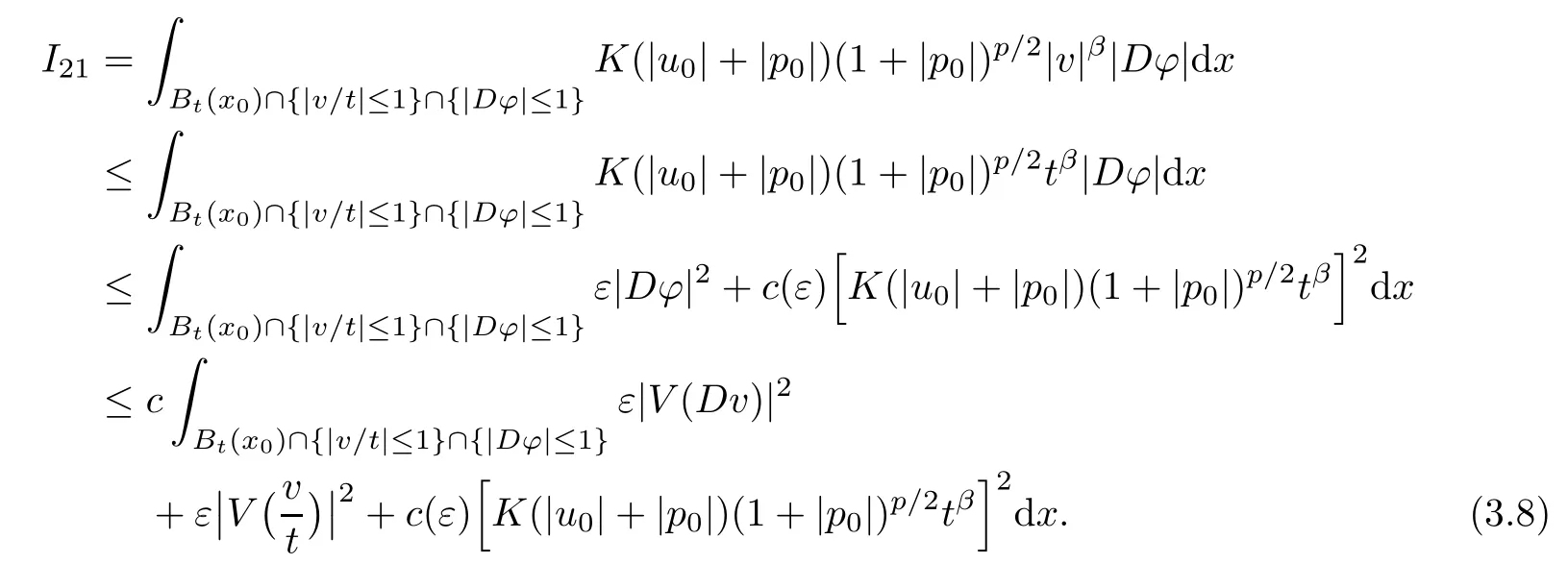
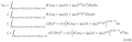
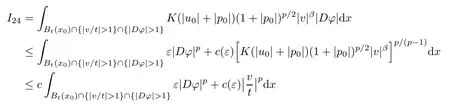
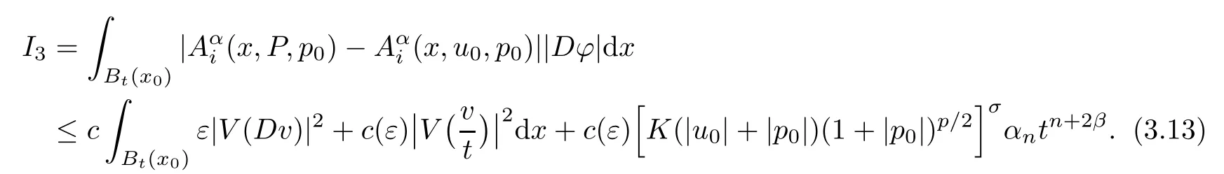
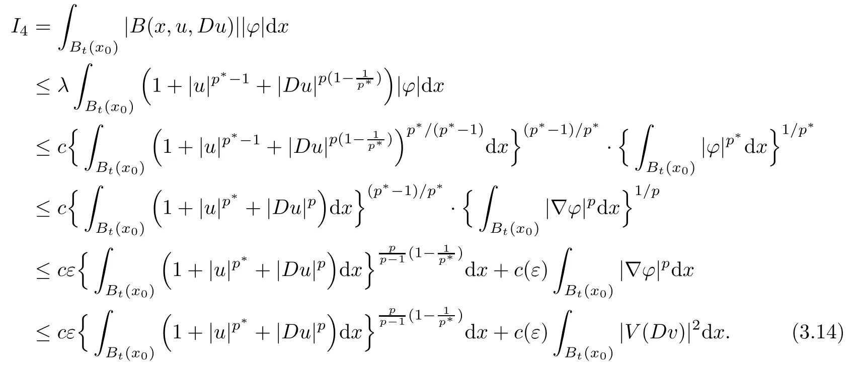
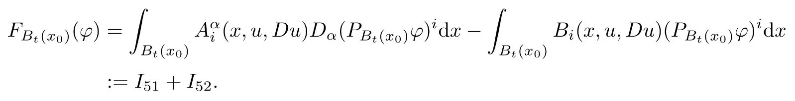
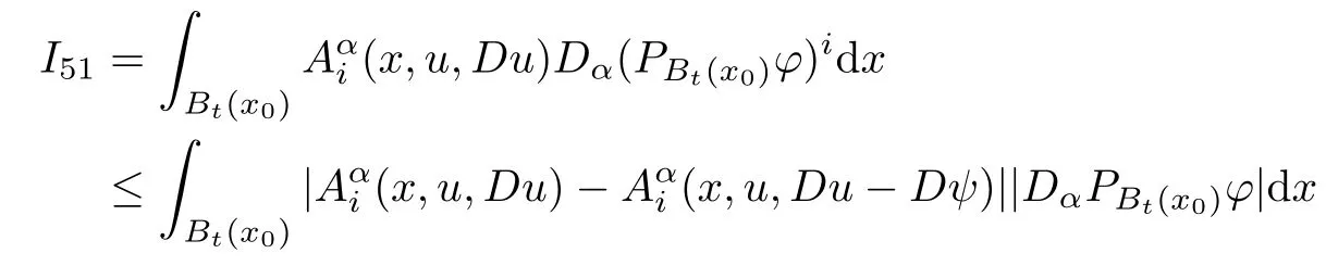
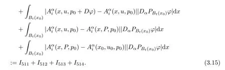
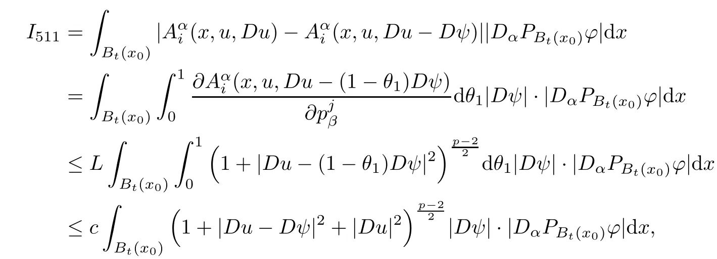
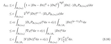
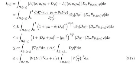
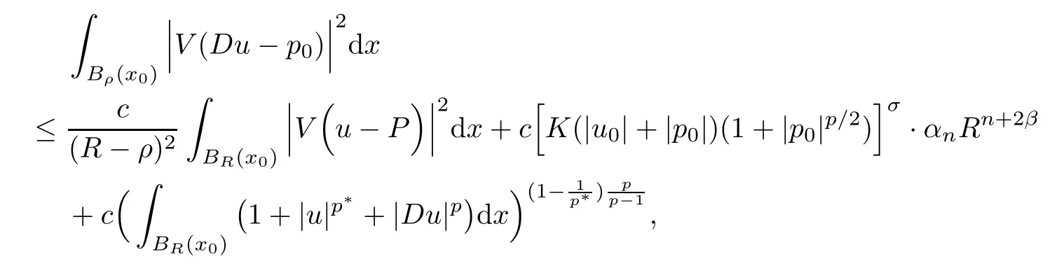
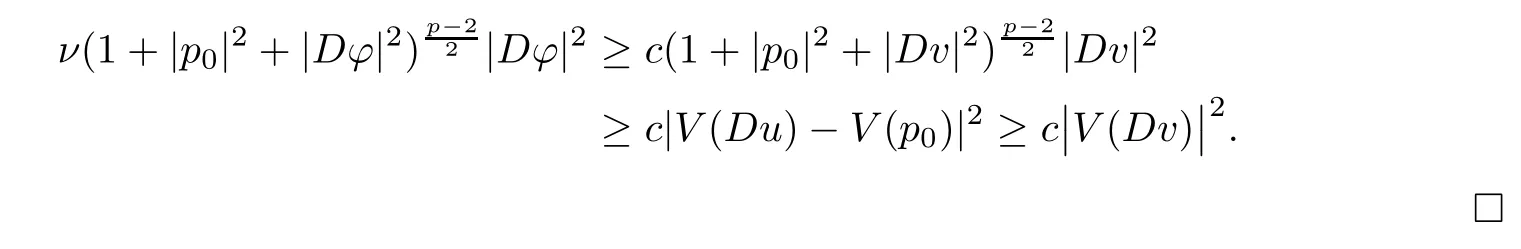
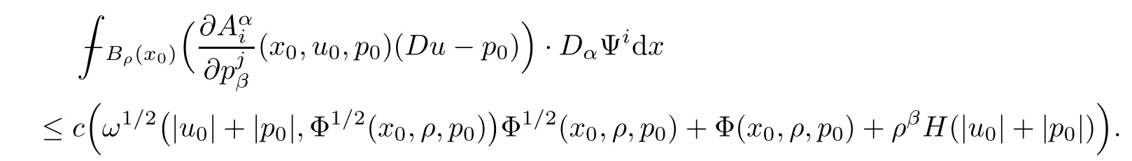
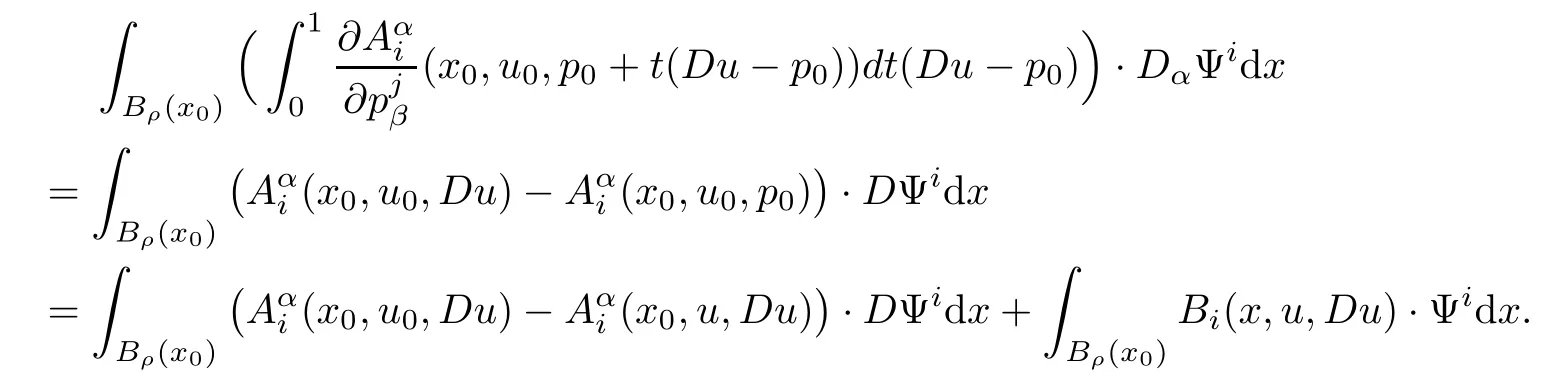
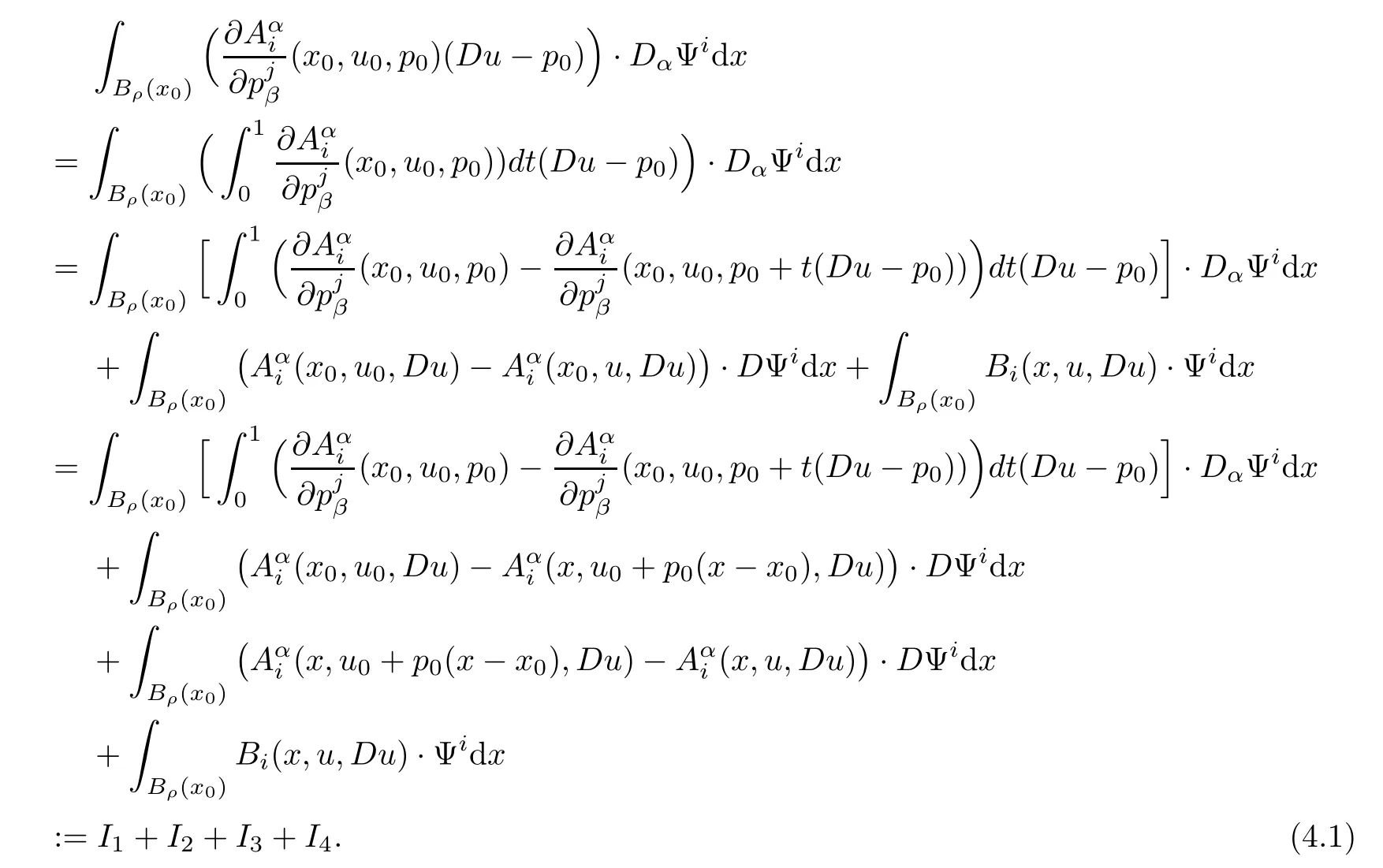
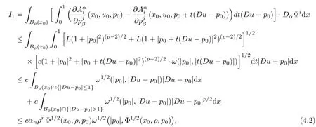
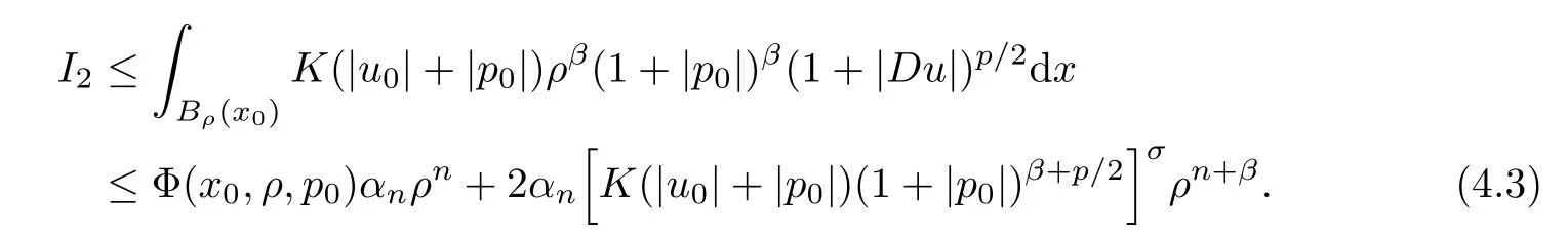
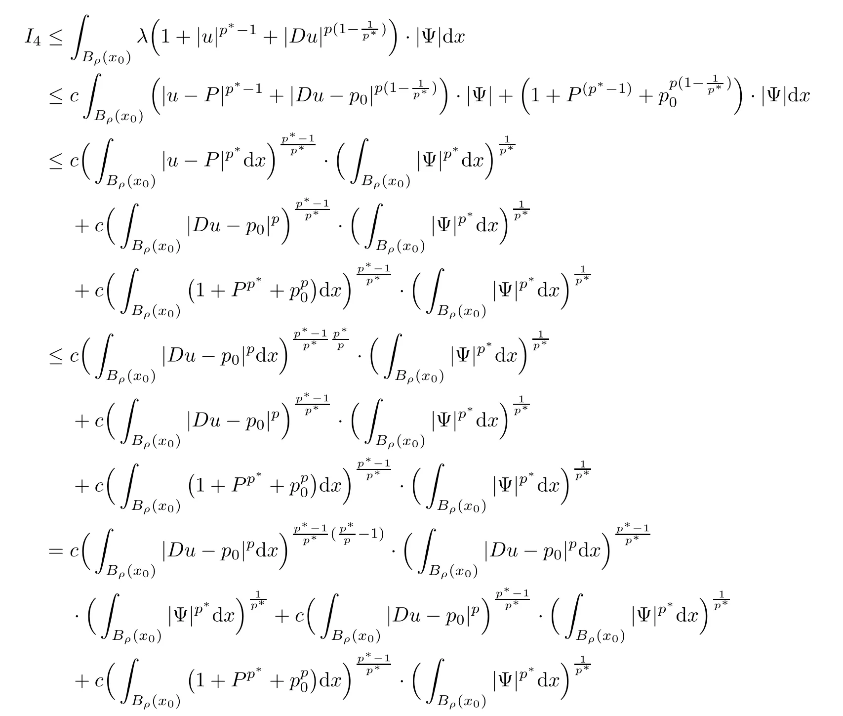
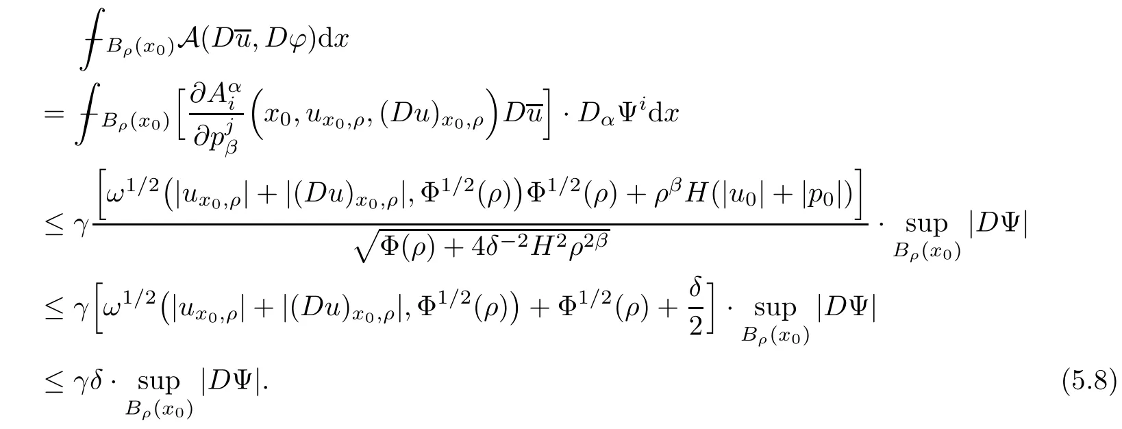
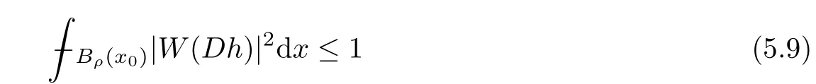
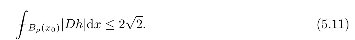
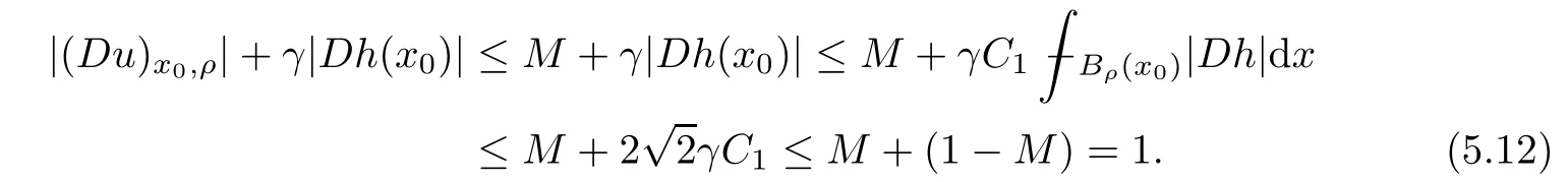
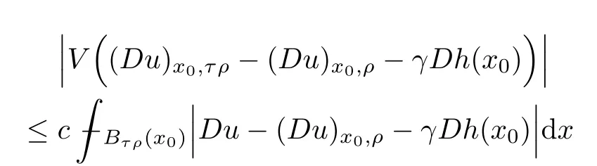
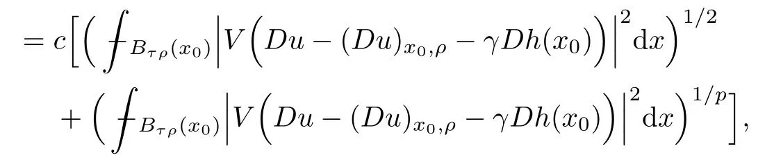
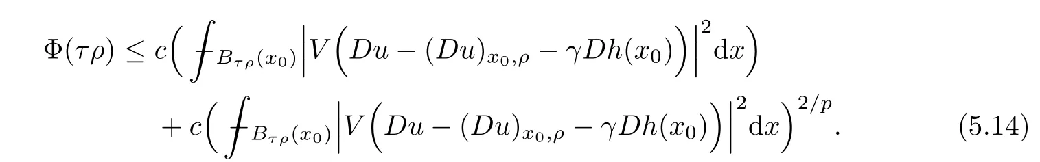
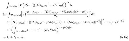
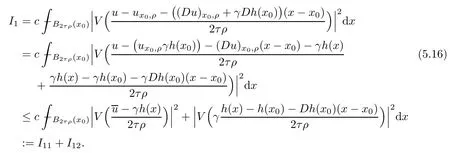
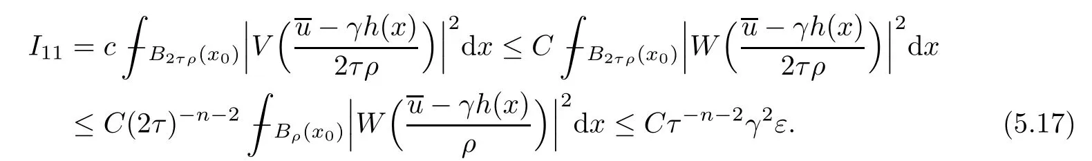
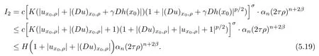
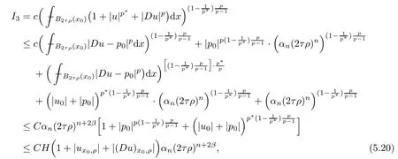
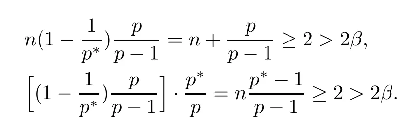
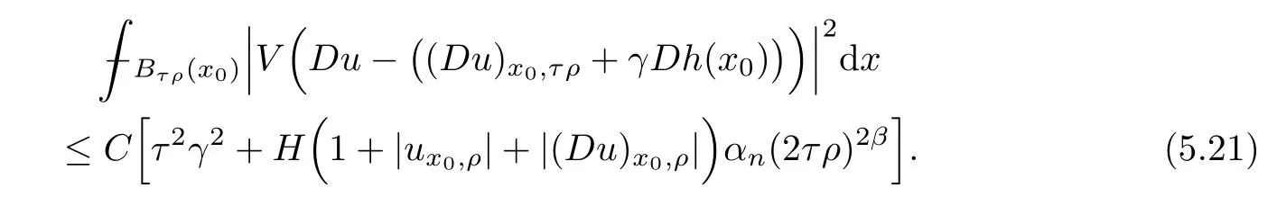
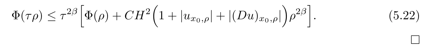
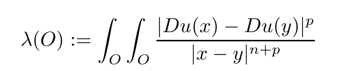
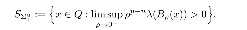
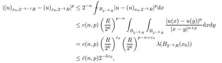
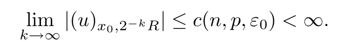
Lemma 2.2For every 1 for any A,B ∈Rk. Here, we state an A-harmonic approximation lemma. Its proof can be found in [14]. We consider bilinear forms A on RNnthat are positive and bounded in the sense for all ξ, η ∈RNn. Definition 2.3A map h ∈W1,1(BR(x0),RN) is called A-harmonic if it satisfies the following linear parabolic system Lemma 2.4Let ν and L be two positive constants. Assume that A is a bilinear form on RNnwith the properties (2.3) and∈W1,p(Bρ(x0),RN) is approximately A-harmonic in the sense Then, for any ε>0, there is a δ >0, depending on p, n, N, ν, L, and ε, and an A-harmonic map h such that and Next, we recall a simple consequence of the a prior estimates for solutions of linear elliptic systems of second order with constant coefficients;see[5](Proposition 2.10)for a similar result. Lemma 2.5Assume that h ∈W1,1(Bρ(x),RN) satisfy where the constant C1depends only on n, N, κ, and K. We state a Poinc´are-type inequality involving the function V,which can be found in[5,14]. Lemma 2.6(Poinc´are-type inequality) Let 1 where p′=2n/(n −p). In particular, the previous inequality is valid with p′replaced by 2. Next, we state a useful elementary lemma. Its proof can be found in [19]. Lemma 2.7For R0< R1, we assume that f : [R0,R1] →[0,∞) is a bounded function and, for all R0<σ <ρ for nonnegative constants A, B, α, and ϑ ∈(0,1). Then, we have the estimate for all R0<σ0<ρ0 Finally, we state two lemmas which will be used to estimate the Hausdroff dimension of the singular set. Lemma 2.8([22, 4.2]) Let u ∈Wθ,p(Br(x0),Rn), where p ≥1, θ ∈(0,1), and Br(x0)⊂RN. Then, we have, for a constant c=c(n,q), Lemma 2.9([22, Section 4]) Let Ω be a open set in Rn. Let λ be a finite, non-negative,and increasing function defined on the family of open subsets of Ω which is also countably superadditive in the following sense that whenever {Oi}i∈Nis a family of pairwise disjoint open subsets of Ω. Then, for 0 < α < n, we have dimH(Eα)≤α, where The first step in the proof of partial regularity is to establish a Caccioppoli type inequality,prepared for decay estimate in Section 5. The precise statement is as follows. For x0∈Ω, u0∈RN, and p0∈RNn, we define P =P(x)=u0+p0(x−x0). Theorem 3.1Let u ∈W1,p(Ω,RN) with ∇·u = g be a weak solution of system (1.1),satisfying (A1) to (A3) and the controllable growth condition (B1). Then, for arbitrary ρ and R with 0<ρ where σ =max{2p/(p −2β),p/(p −1 −β)} and 0<β Here, the constant c depends only on n, N, p, L, λ, and ν. ProofLet 0 < ρ ≤s < t ≤R and choose a standard cut off function ς ∈(Bt(x0))with ς ≡1 in Bs(x0), 0 ≤ς ≤1 and |Dς|≤. Let ϕ and ψ be two test functions satisfying where v =u(x,t)−P(x)=u −u0−p0(x −x0), such that Because supp Dψ ⊂BtBs, we have A straightforward calculation shows that, using the ellipticity condition (A1) stated in the Section 1 and Lemma 2.2, respectively, we have Then, we infer that where Next, we successively deal with the estimation of the terms I1to I5. Here, we consider that so that Combining assumption (A3), estimates (3.2), (3.5) and Young’s inequality, we imply that From (A3), we arrive at In order to estimate it, we split the domain of integration into four parts as which are written by I2≤I21+I22+I23+I24. For the first term I21, we infer by Young’s inequality Secondly, we arrive at Similarly, Combining (3.7) to (3.11), we deduce that where σ =max{2,2p/(p−2β),p/(p −1),p/(p −1 −β)}=max{2p/(p−2β),p/(p −1 −β)} and 0<β Similarly as I2, we arrive at The term I4can be estimated by Hölder’s,Sobolev’s,and Young’s inequalities,respectively. Finally, we deal with I5as First of all, we decompose the term I51into For the term I511, we use assumption (A2) and Lemma 2.2, that is, where Du−(1−θ1)Dψ =Du−Dψ+θ1Dψ =(Du−Dψ)+θ1(Du−(Du−Dψ)):=A+θ1(B−A). Recalling estimate (3.5), we use the fact that supp Dψ ⊂BtBsand Young’s inequality Similarly, the term I512, we use assumption (A2) and Lemma 2.2 to obtain where p0+θ2Dϕ=p0+θ2(Dϕ+p0−p0):=A+θ2(B −A). The terms I513, I514, and I52are similar as I2, I3, and I4, respectively. Recalling (3.4),(3.6), and (3.12)–(3.17), we arrive at where we used Lemma 2.1 to imply In this Section, we apply a linearization argument which will be useful to prove that the weak solutions of systems (1.1) are approximately A-harmonic provided their excess is small.This result is also prepared for decay estimate in Section 5, where we used the A-harmonic approximation lemma. Definition 4.1We define excess functionals Lemma 4.2Let u ∈W1,p(Ω,RN)with ∇·u=g be a weak solution of (1.1). We consider ρ<1 and Furthermore, we fix p0in RNnand set, then, ProofNote that Then, we have For the first term I1, we distinguish the case of |Du −p0| ≤1 and |Du −p0| > 1. We employ assumption (A2), (A4), and Lemma 2.2 with the result where we used the Hölder’s inequality and Jensen’s inequality. Next, we estimate I2with the help of the continuity assumption(A3), the Lemma 2.1,and Young’s inequality by Similarly, we split the domain of integration into four parts as We can derive by Lemma 2.1 Finally, for the term I4, we use a fact that, Hölder’s, Sobolev’s, and Young’s inequalities, then obtain Putting together (4.2)–(4.5) and recalling the definition of H(t), we infer from (4.1) that In this Section, we establish an initial excess-improvement estimate by assuming that the excess Φ(ρ)is initially sufficient small. And we characterize the singular set of the solution with the help of the crucial decay estimate. Lemma 5.1(Excess-improvement estimate) We assume that the hypotheses listed in Section 1 are in force and M > 0. For any weak solution u ∈W1,p(Ω,RN)∩L∞(Ω,RN) of(1.1) with ∇·u=g, if it satisfies the followings: then, we have Proof Step 1We set and Then, we take δ ∈(0,1) to be corresponding constant from the A-harmonic approximation lemma, that is Lemma 2.4. According to (2.2) and Lemma 2.1, we imply Moreover,we can derive, by Lemma 4.2 and the smallness condition (5.2) and (5.3), that With these two estimates (5.7) and (5.8) that satisfies the hypotheses of the A-harmonic approximation stated in Lemma 2.4, there exists an A-harmonic function h ∈W1,p(Bρ(x0),RN)with and Now, with the help of (5.10) and Lemma 2.1, we similarly distinguish the cases |Dh| > 1 and|Dh|≤1 to infer Furthermore, recalling the assumption of (5.1) and Lemma 2.5, we arrive at The estimates (5.10)–(5.12) will be useful in the next step of proof. Step 2We can deduce, with the help of Lemma 2.1, that We note that where we used Lemma 2.1 and decomposed Bτρ(x0) into and Furthermore,we draw a conclusion from(5.13), Lemma 2.1,and the fact that |V(A)|=V(|A|)and t →V(t) is monotone increasing, that is, Applying Theorem 3.1,that is,Caccioppoli type inequality on B2τρ(x0)with ux0,ρand(Du)x0,ρ+γDh(x0) in place of u0and p0, respectively, we have To estimate the first term I1, we use Lemma 2.1 to obtain Here, we draw a conclusion from (2.2), (5.10), and Lemma 2.1, For the second term I12, applying Taylor’s theorem to h on B2τρ(x0), Lemma 2.1, Lemma 2.5,and (5.11), then we have Next, we deal with the term I2by (5.12), Finally, we use assumption (5.4) and Sobolev’s inequality to obtain Combining all the above estimates from (5.15) to (5.20), we arrive at As a result, we deduce (recalling that (5.14)) that The regularity result then follows from the fact that this excess-decay estimate for any x in a neighborhood of x0. By this estimate and Campanato’s characterization of Hölder continuous[4], we conclude that V(Du) has the modulus of continuity ρ →Φ(x0,ρ) by a constant times ρ2β. Furthermore, this modulus of continuity carries over to Du. Finally, we prove that the Hausdorff dimension of the singular set is less than n −p, which follows from [15, Proposition2.1]. We consider a function u ∈W1,p(Q,RN) and a set-function λ defined by on every subset O ⊂Q. Obviously, all the assumptions on λ in Lemma 2.9 are fulfilled. To estimate the Hausdorff dimensions ofand, we define Now let ε>0. Then, Lemma 2.9 implies Hn−p+ε()=0. By Lemma 2.8, we conclude that if x0∈, then x0∈, and therefore,and Hn−p+ε()=0. Again, it follows that Hn−p+ε(SΣu2) = 0 from Lemma 2.9. To prove, we consider centres x0∈QSΣu2and radii R <1 such that BR(x0) ⊂Q. Then, we use Jensen’s inequality and Lemma 2.8 to estimate that for every k ∈N0sufficiently large. Summing up these terms finally yields Hence, because ε0∈(0,ε) is chosen arbitrarily,we obtain Hn−p+ε()=0. So, the Hausdorff dimension of the singular set is less than n −p.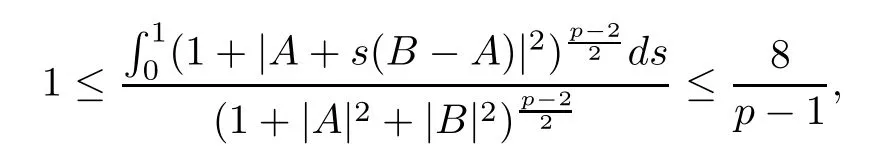
2.2 A-harmonic approximation


2.3 Poinc´are-type inequality
3 A Caccioppoli Type Inequality


3.1 Estimate for I1
3.2 Estimate for I2


3.3 Estimate for I3
3.4 Estimate for I4
3.5 Estimate for I5
4 Approximate A-Harmonicity by Linearization


4.1 Estimate for I1
4.2 Estimate for I2
4.3 Estimate for I3
4.4 Estimate for I4
5 A Decay Estimate


5.1 Estimate for I1
5.2 Estimate for I2
5.3 Estimate for I3

 Acta Mathematica Scientia(English Series)2020年3期