A New Temperature Channel Selection Method Based on Singular Spectrum Analysis for Retrieving Atmospheric Temperature Profiles from FY-4A/GIIRS
Peipei YU, Chunxiang SHI, Ling YANG, and Shuai SHAN
1College of Electronic Engineering, Chengdu University of Information Technology, Chengdu 610225, China
2CMA Key Laboratory of Atmospheric Sounding, Chengdu 610225, China
3National Meteorological Information Center, Beijing 100081, China
4College of Geographic Sciences, Nanjing University of Information Science and Technology, Nanjing 210044, China
ABSTRACT Hyperspectral data have important research and application value in the fields of meteorology and remote sensing.With the goal of improving retrievals of atmospheric temperature profiles, this paper outlines a novel temperature channel selection method based on singular spectrum analysis (SSA) for the Geostationary Interferometric Infrared Sounder(GIIRS), which is the first infrared sounder operating in geostationary orbit. The method possesses not only the simplicity and rapidity of the principal component analysis method, but also the interpretability of the conventional channel selection method. The novel SSA method is used to decompose the GIIRS observed infrared brightness temperature spectrum(700−1130 cm−1), and the reconstructed grouped components can be obtained to reflect the energy variations in the temperature-sensitive waveband of the respective sequence. At 700−780 cm−1, the channels selected using our method perform better than IASI (Infrared Atmospheric Sounding Interferometer) and CrIS (Cross-track Infrared Sounder)temperature channels when used as inputs to the neural network retrieval model.
Key words: infrared hyperspectral data, temperature channel selection, singular spectrum analysis, temperature profiles retrieval
1. Introduction
An important means of understanding complex atmospheric systems is to take advantage of vertical profiles,such as those for temperature. Together with conventional observational data, vertical profiles can provide an accurate initial field for numerical prediction models. Conventional temperature profile data usually come from radiosondes(Luers and Eskridge, 1998; Divakarla et al., 2006).However, it is not possible to obtain higher frequency observations because radiosonde data are usually available twice a day and the radiosonde stations are separated by about 300 km. Infrared hyperspectral sounders, such as AIRS(Atmospheric Infrared Sounder), CrIS (Cross-track Infrared Sounder), and IASI (Infrared Atmospheric Sounding Interferometer), are mounted on polar-orbiting satellites. In contrast,the Geostationary Interferometric Infrared Sounder (GIIRS)onboard the Fengyun-4A (FY-4A) satellite is the first infrared hyperspectral sounder operating in a geostationary orbit, and therefore has the advantage that it provides nearreal-time tracking and forecasting of extreme weather events with a higher spatial and temporal accuracy than the instruments on polar-orbiting satellites (Yang et al., 2017).Considering the large amount of spectral data generated by GIIRS, how to compress the dataset while retaining the significant information content is crucial.
A widely used solution is to reduce the dimension of the data—an approach that is generally divided into two kinds of strategies (Aires et al., 2016). The first is feature extraction—a technique performed on the entire waveband to extract the most representative features. Principal component analysis (PCA) is recognized as an efficient tool for dimensionality reduction (Huang and Antonelli, 2001; Serio et al., 2018). Analogous to the discrete version of the Karhunen−Loeve transform, PCA is provided by the singular value decomposition (SVD) theorem applied to the covariance matrix of the given process. In the field of remote sensing and satellite meteorology, PCA is usually called empirical orthogonal function (EOF) analysis. First exploited by Wark and Fleming (1966), the application of PCA/EOF then flourished in many applied research fields, such as data assimilation, the estimation of physical parameters and trace gases (Chahine, 1970), the radioactive transfer equation inverse problem in the component space (Smith, 1970), and temperature profile retrieval from high spectral resolution infrared data (Blackwell, 2005). Another strategy for dimensionality reduction is channel selection—a method that selects a portion of the value from the observation sequence whilst retaining the original values as much as possible according to certain selection criteria. A typical example is its use to select channels on infrared hyperspectral sounders,such as IASI (Collard, 2007; Ventress and Dudhia, 2014;Noh et al., 2017) and CrIS (Gambacorta and Barnet, 2013).This method is able to perform selection by prioritizing the characteristics of the channel, making it more explanatory than the feature extraction method. Thus, for a specific field such as that of a trace gas, or for temperature profile retrievals, it is a more efficient method than feature extraction.
However, both methods have their limitations. A general limitation of the basic PCA method is the determination of the extent of approximation. PCA attempts to reduce data dimensionality by maximizing the variance of the first principal component, ignoring multiple potential variables or information (Aires et al., 2016). The rapidity and simplicity make PCA appealing, although the physical interpretation of the method is not always clear. In contrast, channel selection has better interpretability based on selection criteria. However, the selection criteria may cause only the variables with higher values in the selected channel subset to be focused on, and variables with lower values ignored.
The aim of this paper is to select channels for the specific application of temperature profile retrieval. Both strategies mentioned above select channels based on the entire spectrum, either by extracting some features to represent the entire spectrum, or by specifically selecting some channels from the entire spectrum. However, in some cases, only the most interesting channel need be selected.
We propose a novel channel selection method by combining singular spectral analysis (SSA) and standard deviation(SD) threshold detection on the grouped components reconstructed by the SSA, in order to separately select the temperature channels of GIIRS for the specific application of temperature profile retrieval. The SVD processing used in basic SSA is similar to the PCA method; the main difference is that SVD uses the property of the Hankel structure of the trajectory matrix (Hassani, 2007), while PCA does not. In general,SSA is a useful tool for dealing with time series, including the forecasting of interannual variation in the climate system (Biondi et al., 2001; Hansen et al., 2011), and missing value imputation (Ghafarian Malamiri et al., 2018). In addition, SSA can also be used for data preprocessing of models, such as feature extraction (Zabalza et al., 2015; Liu et al., 2018) or data augmentation on the input data of neural networks (Wu and Chau, 2011; Gao et al., 2016).
In our method, the GIIRS infrared brightness temperature spectrum can be regarded as a time series sequence and the SSA method used to decompose and reconstruct components of it. We use the clustering method to obtain each cluster’s central sequence, the most representative sequence of a cluster, which are subsequently used for channel selection. Here, a cluster is a set of objects (brightness temperature spectra) in which each object is closer (or more similar)to every other object in the cluster than to any object not in the cluster. The temperature channel subset is selected from the grouped components of the central sequence using the SD of the corresponding grouped component as a threshold to select temperature channels in the temperature sensitive band. The channel subset is then compared with other temperature channel subsets to verify the performance of the retrieval when used as an input to the neural network model.
The remainder of this paper is organized as follows: Section 2 introduces the GIIRS data and the radiosonde data. Section 3 describes the methods of data matching, channel selection with the combination of the clustering method, the SSA and variance threshold detection method for the GIIRS infrared brightness temperature spectrum, and the neural network model for the retrieval. Section 4 describes the experimental process of channel selection using the new method,and the setting of the Artificial Neural Network (ANN)model. Section 5 describes the results of the final temperature channel subset of GIIRS with a comparison of other subsets, and the results of the performance of retrieving temperature profiles. Finally, conclusions are presented in section 6.
2. Datasets
2.1. FY-4A GIIRS data
GIIRS is one of main instruments onboard China’s second-generation geostationary meteorological satellite,FY-4A, which was launched on 11 December 2016. It is the first precise remote sensing instrument in geostationary orbit, detecting the vertical structure of the three-dimensional atmosphere via infrared hyperspectral interference spectroscopy (Menzel et al., 2018). The primary task of GIIRS is to measure the distribution of temperature and humidity in the atmosphere. As the first hyperspectral sounder mounted on a geostationary satellite, GIIRS complements the observations of sounders on polar-orbiting satellites, providing almost continuous temporal, horizontal and vertical observations, which are especially useful for regional nowcasting and tracking extreme weather events.
GIIRS uses the Fourier transform to recover the atmospheric absorption spectrum with high spectral resolution.It covers the range of the long-wavelength band (700−1130 cm−1), the mid-wavelength band (1650−2250 cm−1),and the visible light band (0.55−0.75 μm). The detectors at the two infrared wavebands both have 32 × 4 sensor elements. There are a total of 1650 infrared channels, of which 689 are for the long-wavelength band and 961 for the midwavelength band. The spectral resolution of the long- and mid-wavelength bands is 0.625 cm−1. The spatial resolution of the infrared and visible bands is 16 km and 2 km, respectively, and the temporal resolution is 67 min (for the China area). Table 1 lists the main performance characteristics of GIIRS.
The observational area of GIIRS in China is not fixed,but rather is based on the requirements of the Numerical Weather Prediction Center of the China Meteorological Administration (CMA). Unlike IASI, GIIRS does not perform long continuous detection on the waveband, but rather divides the spectral range into the two wavelength bands.Therefore, referring to the retrieval method of GIIRS Level-2 (L2) temperature profile products, the channel selection method proposed in this paper focuses only on the longwavelength band, with GIIRS Level-1 data (clear-sky) from August 2018 to November 2018 selected.
2.2. China radiosonde data
The high resolution radiosonde data used in this study are from the China Integrated Meteorological Information Service System of the CMA. The L-band (1675 MHz) sounding radar is a new generation of secondary wind-measuring radars, which are fully automated in China and synchronized with GTSl digital electronic radiosondes (Zeng et al.,2019). It is widely used to measure the air temperature, pressure, relative humidity, and wind from the ground to about 30 km in operational radiosonde stations in China. During the balloon launching process, the sounding data were collected approximately every 1.2 s and the accuracy of the measured temperature, pressure, and humidity is 0.2°C −0.3°C,1−2 hPa, and 4%−5%, respectively (CMA, 2010). Compared with the previous radiosonde, Model 49, and secondgeneration radiosonde, Model 59, the data acquisition rate,accuracy, and reliability of the L-band radiosonde are significantly better and the GTS1 radiosonde temperature detection accuracy is comparable to the Vaisala RS80 and RS92 radiosondes. There are 120 L-band upper-air sounding systems in China, all of which provide Level-2 sounding data at 0000 UTC and 1200 UTC daily, according to the demand for high-altitude observations, in addition to encrypted observation at 0600 UTC and/or 1800 UTC depending on weatherconditions or detection experiments.

Table 1. Key GIIRS parameters.
Radiosonde data used in this paper have undergone strict quality-control procedures by the National Meteorological Information Center of the CMA, including missingdata inspection, station climatological limit value inspection, vertical consistency checks, duplicate value checks,and internal consistency checks (Yuan et al., 2016). Corresponding to the Level-1 radiance data of GIIRS, radiosonde data from August 2018 to November 2018 were selected and include conventional observation data and encrypted observation data. The radiosonde data were used as true values to test the performance of the temperature profile retrieval model.
3. Methods
3.1. Data matching
Before implementing data matching, each radiance value detected by GIIRS should be converted to a brightness temperature value according to the inverse Planck function:

where t is the blackbody temperature (K), Lbris the blackbody radiance (mW m−2sr−1cm), c1= 119104.2(mW m−2sr−1cm4), c2= 1.4387752 (K cm−1) and v is the wavenumber (cm−1).
Then, the coordinate of each detector unit (latu, lonu) is matched with that of each L-band sounding station (lats,lons). By setting a threshold of distance on the surface of a sphere, sample pairs [(latu, lonu), (lats, lons)] that meet the following distance threshold criterion can be obtained:

where R represents the radius of the Earth (6371 km). The distance threshold is set according to the spatial resolution of GIIRS.
In addition to spatial matching, the observation time is also considered. Starting from the ground, it takes about 75 min for the sounding balloon (flight time starts at 2315 UTC, 1115 UTC, 0515 UTC or 1715 UTC) to reach a height of about 30 km (CMA, 2010). The temperature profile may simultaneously match multiple brightness temperature spectra during the balloon’s detection time. Based on the consideration of neural network robustness, these samples are preserved for training. After spatial and temporal matching, a total of 9734 sample pairs were selected.A brightness temperature spectrum detected by GIIRS corresponds to a temperature profile obtained by a radiosonde.
For each brightness temperature spectrum, we defined a range of 150−350 K to ensure its validity. Thus, any value outside this range was excluded. For sounding temperature profiles, due to the vertical resolution varying from station to station, and from sounding to sounding at the same radiosonde station, we required a more demanding selection. According to statistical analysis of the profile, we further selected the effective data for pressure levels in the range 100−900 hPa,which cover most areas in China except the Qinghai−Tibet Plateau and ensure the consistency of output layers in retrieval validation models. We then performed linear interpolation based on the detection accuracy (0.1 hPa) of the pressure level to obtain the corresponding temperature value at each level. Finally, some pressure levels [900 hPa, 875 hPa,850 hPa, 825 hPa, 800 hPa, 775 hPa, 750 hPa, 700 hPa, 650 hPa, 600 hPa, 550 hPa, 500 hPa, 450 hPa, 400 hPa, 350 hPa, 300 hPa, 250 hPa, 225 hPa, 200 hPa, 175 hPa, 150 hPa, 125 hPa, 100 hPa] in this range were selected based on the pressure levels in the ERA5 reanalysis data.
A total of 5021 sample pairs met the requirements of the data matching and preprocessing stages. The results of the above process are shown in Fig. 1. The GIIRS infrared brightness temperature spectra in this dataset were used for channel selection and in the neural network models with the corresponding sounding temperature profiles. The specific data usage will be explained in the respective sections.
3.2. Temperature channel selection
3.2.1. Brightness temperature spectrum clustering
We consider the brightness temperature spectrum as a time-like sequence because it reflects continuous spectral information. We first clustered the brightness temperature spectrum samples using the k-means++ clustering method(Arthur and Vassilvitskii, 2007), extracting the central sequence samples for each cluster to represent the overall characteristics of each cluster for the SSA. The k-means++clustering method is a variant of the k-means clustering method, which can effectively avoid the problem of poor performance on clustering and slow convergence due to random selection of the center point (Arthur and Vassilvitskii,2007). The preset cluster number k has the range [0, 10],and the sum of the squared error (SSE) under different k values was calculated according to the following formula to obtain the optimal number of clusters:

where k is the number of clusters, Ciis the ith cluster, p is a point of Ci, and miis the mean of all points in Ci.
3.2.2. SSA

Fig. 1. Geographic distribution of radiosonde stations (120) of the CMA and the results of data matching. In total, 79 radiosonde stations (red dots) met the data matching requirements.The scatter size (red dots) corresponds to the number of matched sample pairs.
The SSA method can decompose a sequence into multiple components reflecting different implicit information,such as local energy variation and periodic variation in the original sequence (Hassani, 2007; Golyandina and Zhigljavsky,2013). Suppose we have a central sequence S = (s1, s2, …,sN) with length N. Convert S to a trajectory matrix X consisting of lagged vectors with window length L. Then, the SVD of the trajectory matrix X can be written as X=X1+X2+...+Xd, where d = rank(X) can be regarded as the intrinsic dimensionality of the sequence’s trajectory space, and Xiis the elementary matrix of X. After diagonal averaging performed on each elementary matrix, the original sequence S corresponding to X can be converted to a form superimposed by different components, as below:

where Yi(i=1,2,...,d) can be considered the ith component of S. The length of each component is equal to that of the original sequence S.
Next we use w-correlation to measure the correlation between the components and divide the components with high correlation into one group. For two components of length N, Yiand Yj, and window length L, we define the weighted inner product as

where yi,kand yj,kare the kth values of Yiand Yj, respectively, and wkis given by

The weight wkreflects the number of times yi,kand yj,kappear in the trajectory matrix X of the sequence S. If(Yi,Yj)w=0, the components Yiand Yjare considered worthogonal. In the real word, total w-orthogonality does not exist, so instead we define a w-correlation matrix, Wcorr,which measures the degree of the approximate separability between Yiand Yj. The elements of Wcorrare given by


where Yi(i=1,2,...,m) is the ith grouped component of S.
3.2.3. Channel selection
Channel selection for hyperspectral data can be highly beneficial both to improve the predictive ability of the model and to greatly enhance its interpretation. However,the main difficulties are not only that consecutive variables in the spectrum are highly correlated by nature, but in addition real applications usually concern databases with low numbers of known spectra, and a high number of spectral variables. The purpose of performing SSA on a brightness temperature spectrum is to find the implied information of temperature that is not easily found in the brightness temperature spectrum, but rather in the grouped components of it. The grouped components can be interpreted as the filtered and amplified results of the brightness temperature spectrum corresponding to specific requirements, such as corresponding to temperature-sensitive bands. The difference between each grouped component is maximized, ensuring that the channels selected from each grouped component have their own representatives. For the case where the information represented by each grouped component is different, we adopt a method based on each grouped component’s SD to select channels adaptively. The SD is a measure of how far the grouped component fluctuates from the mean, and the variance (SD2) represents the power of this fluctuation. Then,we combine the channels together as the final channel subset of this sequence. For a grouped component Y=(y1,y2,...,yn):
(1) Calculate the SD and use it as a threshold by

where yi(i=1,2,...,n) is the ith value of Y andis the mean of these values, while N is the length of Y.
(2) Find the extrema, including the maxima and minima. A point ymof Y is an extremum if there are adjacent indices i and j, where i < m < j, such that ym(maximum)strictly satisfies yi< ymand ym> yj, or ym(minimum) strictly satisfies yi> ymand ym< yj. All extrema of Y, called feature points, will be further selected by the SD threshold and satisfy ym> SD or ym< −SD.
By using the SD as a threshold for screening, we obtain the indices of the feature points of this grouped component,with each index corresponding to its respective wavenumber, and will be considered as a channel used to retrieve temperature profiles. The channels of other grouped components can also be selected following the same procedure.
3.3. ANN
ANNs are widely used in nonlinear regression (Feng et al., 2017; van Gerven and Bohte, 2017) and pattern recognition models (Iglovikov et al., 2017). Many researchers are also using ANNs and their variants to retrieve atmospheric parameters (Blackwell, 2005; Chakraborty and Maitra,2016; Whitburn et al., 2016) or surface parameters (van Damme et al., 2017; Ge et al., 2018). The ANN retrieval method does not aim to explicitly formulate the physical processes linking the satellite observations to the atmospheric state, but instead creates a model of the nonlinear statistical relationship between them. Contrary to the Radiative Transfer Model, an ANN does not rely on knowledge of the physical processes and requires less a priori knowledge of the atmospheric characteristics and radiative transfer parameters. Instead, it provides the best model to combine the atmospheric information provided by the satellite data inputs(Kolassa et al., 2017). In light of the above, a typical neural network with a single hidden layer is used to validate the performance of the temperature profile retrieval, with the final channel subset as its input. There are 23 fixed output nodes,each of which corresponds to the temperature value of a pressure level. The min-max scaling method was used to normalize inputs/outputs to fall in the range [−1, 1]. Nodes in the hidden and output layers apply the sigmoidal activation function and linear activation function, respectively. The ANN was trained using the Levenberg−Marquardt back-propagation algorithm (Moré, 1978). Figure 2 shows the model architecture.
The neural network model of the temperature profile retrieval was developed based on a training set and validation set, while the performance of the neural network was evaluated using a testing set. The training, validation, and testing sets comprised 60%, 20%, and 20% of the sample pairs,respectively. The network training stops when the number of validation checks reaches 12, which represents the number of successive iterations above which the validation performance does not increase (Beale et al., 2018). All the nodes of the output layer are combined to produce a complete predicted temperature profile, which is compared with the target (the true temperature profile in the sample pairs of the training set). Each node error can be calculated by

where yiandare the ith target value and retrieved value,respectively.
The performance of the retrieval depends on the architecture of the ANN model—in particular, the number of nodes in the input layer and the hidden layer. The former is determined by different channel subsets, including the temperature channel subset of IASI, CrIS, and our channel subset selected based on the SSA method. The candidate number of hidden layer neurons (Table 2) is based on results from previous studies (Wanas et al., 1998; Shibata and Ikeda, 2009;Beale et al., 2018).
The performance of the retrieval model was quantified using several statistical error evaluation indices, including the mean absolute error (MAE), root-mean-square error(RMSE) and coefficient of determination (R2).
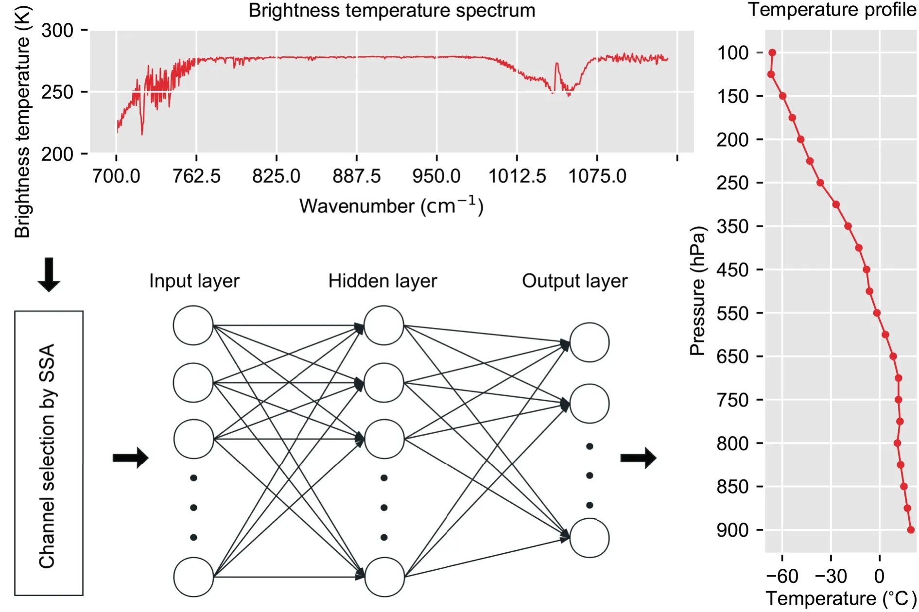
Fig. 2. The architecture of the ANN model. The brightness temperature spectrum sample has 689 channels in the longwavelength band (700−1130 cm−1) with a spectral resolution of 0.625 cm−1. The sounding temperature profile sample has a total of 23 selected pressure levels between 100 and 900 hPa, and each pressure level corresponds to a measured temperature value.

Table 2. Hidden layer neuron settings of the neural network. T is the number of samples used for training, which in this case is 3012.(Nc)i is the number of input nodes, referring to that of the selected temperature channels for CrIS. No is the number of output nodes corresponding to that of the selected pressure levels.
4. Experiments
We first obtained the GIIRS infrared brightness temperature spectrum samples that had been matched with each sounding station observation, and randomly sampled the samples at different observation times from each sounding station in a ratio of one-fifth. If the number of samples from a sounding station at a certain observation time did not exceed five,only one sample of this observation time was selected.Then, we used the min-max scaling method to normalize the selected samples to improve computational efficiency.For each k in [0,10], we initialized k-means++ and used the inertia attribute to identify the SSE of samples to the nearest cluster center. Finally, the value of k was chosen to be 4 and the central sequence of the respective cluster was extracted for channel selection.L to L=floor(689/4)=172, where floor(x)=, and per-
For the SSA, we set the first parameter window length formed SVD on the constructed Hankel matrix. Then, the eigenvalues were arranged in order from largest to smallest together with the corresponding eigenvectors. The corresponding elementary matrices were also obtained.
Figure 3 demonstrates that the contribution rate of the first elementary matrix of C0is almost 99.86%, which means its contribution rate is much larger than the sum from the other components. The sum of the contribution rates of the first 12 elementary matrices of those sequences all exceeded 99.98%, with C2reaching almost 100%. From the perspective of dimensionality reduction, we only show the energy contribution rate of the first 12 elementary matrices of the center sequence of each cluster (Cifor i = 0, 1, 2, 3).
It is assumed that the 12 elementary matrices of C0are all independent after SVD decomposition. According to Eq.(4), the corresponding 12 components are shown in Fig. 4.Starting from Y1, we moved all subsequent components in parallel on the y-axis and the distance between each zero tick on the y-axis was set to 10 K. We can intuitively find that Y0has a value of approximately 250 K, which almost represents the main range of C0. From Y1, the value starts to decrease significantly, and the rest of the components maintain small fluctuations above and below 0. This corresponds to the energy contribution rate of C0in Fig. 4. It can be seen that Y1reflects the general trend of C0. The main variations of Y2−Y4and Y7−Y11are distributed at 1000−1130 cm−1, and values gradually decrease; whereas, the main variations of Y5−Y6are distributed at 700−800 cm−1, and the variation is more severe.
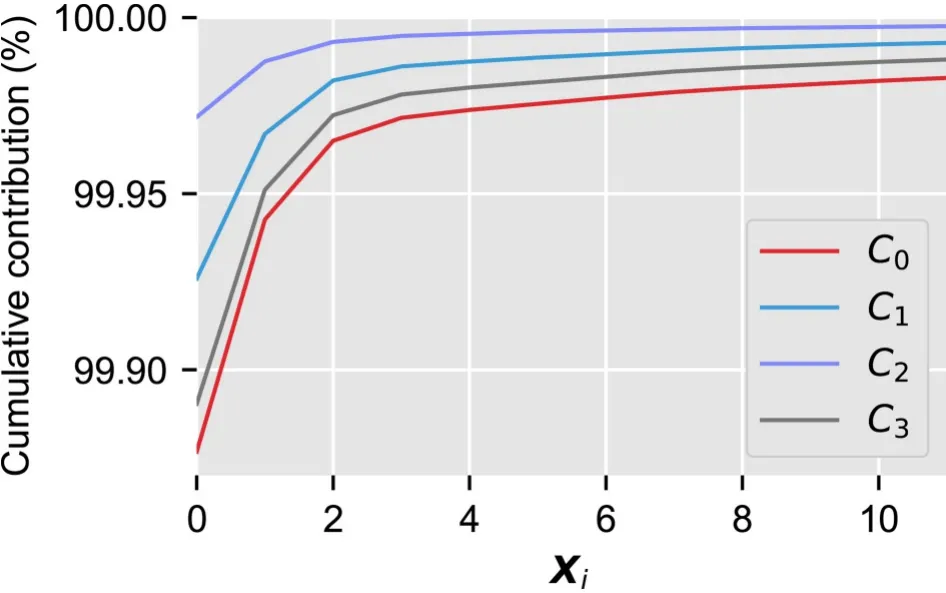
Fig. 3. The cumulative contribution rate (%) of each cluster’s central sequence.
Next, we used w-correlation between components as separability measures. Figure 5 shows the w-correlation matrix for C0, with blue to red colors corresponding to the absolute value of correlation from 0 to 1. The first component,Y0, describes the main trend, and hence it is w-orthogonal to the other components. Moreover, the large sparking square excluding Y0indicates that there is weak separability between those components behind Y0, while attention must be paid to components Y5and Y6whose w-correlation values with each other are almost equal to 1, but approximately zero with other components. This feature implies that we can extract these two components as a separate group. The grouped component composed of the two components that correspond to the elementary matrices X5and X6of X can effectively separate the information of the temperature-sensitive band and enlarge the separation result; thus, it can be regarded as a filter for the specified band.
Based on these results, we then reused w-correlation to analyze the central sequences of the remaining three clusters(Cifor i =1, 2, 3) for comparison (Fig. 6). There are always two highly w-correlated components in each central sequence, and the w-correlation values between these two components and other components is almost zero.
Another phenomenon worth considering is that the two highly w-correlated components of each central sequence are always adjacent. The order of arrangement of these components corresponds to the order of energy contribution rate from largest to smallest. In the case of determining the adjacent characteristics, the order of the energy contribution rates of the two components are not the same. The two components of C0are fifth and sixth in order of energy contribution rate, respectively, while the two components of the others are sixth and seventh. However, we can be sure that the two components all reflect the energy in certain bands, and they are highly w-correlated with each other. Therefore, the common characteristics of these central sequences provide a basis for grouping. That is, the first component is a separate group, the two highly w-correlated components are combined into a second group, and the remaining components are combined into a third group. The first, second and third groups can be called the 1st, 2nd and 3rd grouped components, respectively.
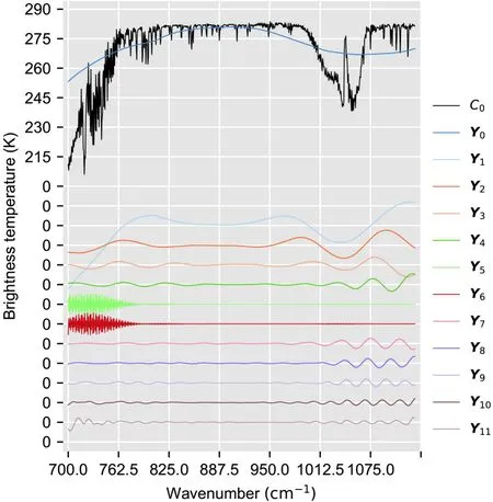
Fig. 4. Decomposing C0 and reconstructing it without grouping. The 12 components correspond to the 12 first elementary matrices of C0.
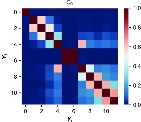
Fig. 5. The w-correlation matrix of C0.
Through the proposed method, we enlarge the energy variation information of the temperature-sensitive band,which is difficult to be seen in the original brightness temperature spectrum from the 2nd grouped component, and adaptively select the temperature channel accordingly. The results of channel selection on grouped components of each central sequence are shown in Fig. 7.
5. Results
5.1. Temperature channel subset of GIIRS
We combined the channels selected by each cluster’s own central sequence to achieve the final channel subset of GIIRS. To verify this subset of channels is available for the retrieval application, we compared it with two other sets of temperature channels—that of IASI and that of CrIS.However, a direct comparison is not trivial, as the IASI temperature channels do not have exactly the same frequencies as those of GIIRS, and the channels were chosen based on different criteria. To aid the comparison, the spectral resolution of GIIRS was linearly interpolated so that it is identical to the spectral resolution of IASI. No processing was required with CrIS because it has the same spectral resolution as GIIRS in the long-wavelength band.
Figure 8 compares the temperature channels selected from GIIRS with those of IASI and CrIS in the range 700−1130 cm−1. The channels outside this interval are excluded, because these channels are not within the longwavelength detection range of GIIRS. The number of channels of GIIRS, IASI and CrIS is 106, 49 and 23, respectively. For GIIRS, there are 89 temperature channels distributed at 700−780 cm−1(Table 3), and 17 temperature channels distributed at 1000−1130 cm−1. The channel subset of GIIRS can reflect more temperature-sensitive information than the other two channel subsets.
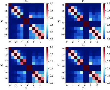
Fig. 6. As in Fig. 5 but with the w-correlation matrices of the central sequences shown together for comparison.
5.2. Retrieval of temperature profiles
The results of the retrieval mainly depend on the model architecture. Specifically, its performance is limited by the setting of the neural network hyperparameters, such as the structure of the network, the optimization algorithm, the number of input and output neurons, and the number of hidden layer units.
Therefore, our neural network model only requires two user inputs. The first is the number of input neurons, which is derived from the different channel subsets, including those selected by SSA, the channel subset of IASI, and that of CrIS. We only used GIIRS temperature channels in the 700−780 cm−1range (Fig. 8) as the network’s input,because there are no comparable temperature channels at 1000−1300 cm−1. The second model parameter to be set is the number of hidden layer neurons (Table 2), which was set based on the empirical formula used in previous studies.In short, the two candidate parameter sets were [89, 49, 23]and [55, 23, 12, 10] for the number of input neurons and hidden layer neurons, respectively. Therefore, a total of 12 models were used to assess retrieval performance. These models were optimally trained by validation checks to prevent overfitting and underfitting, thereby minimizing the model calculation time.
As shown in Fig. 9, the linear regression lines between all predicted and associated true values are close to the bestfit regression lines. Attention must be paid to the spines representing the distribution of the sample spaces, where the two highest peaks of the two curves correspond to each other. This means that for the 23 pressure levels selected,there are two pressure levels and the temperature of each is close to the temperature of the vicinity pressure level. In other words, an interesting piece of information can be obtained: we can judge whether the selected pressure level has a better representation of important changes in a complete temperature profile according to the overall distribution of the sample.
From the distribution of the testing samples, the more neurons in the input and the hidden layers, the closer the samples are to the regression line and the smaller the error between the predicted and true values. Therefore, Fig. 9a shows that the model performs best when the number of input and hidden layers is set as 89 and 55 respectively.Although the best model also produces certain anomalous predictions, these results do not affect the overall performance on the testing set.
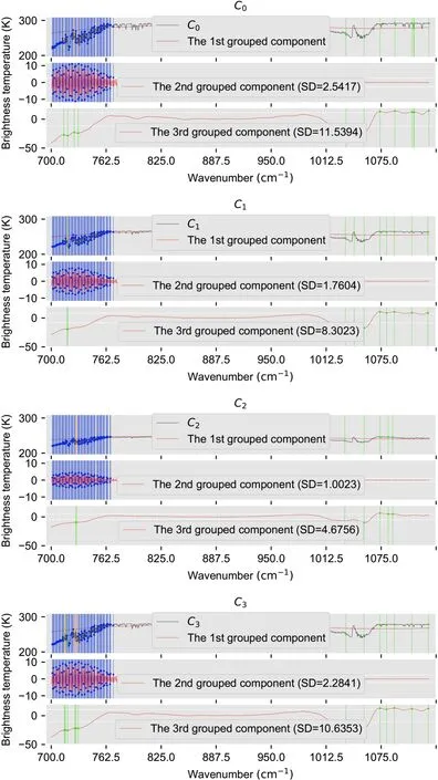
Fig. 7. The results of temperature channel selection on each central sequence. The blue dots represent the feature points selected from the 2nd grouped component, and the green dots represent the feature points selected from the 3rd grouped component. The yellow dots indicate the feature points common to the 2nd and 3rd grouped components. The vertical lines represent the channels corresponding to these feature points detected using the SD.
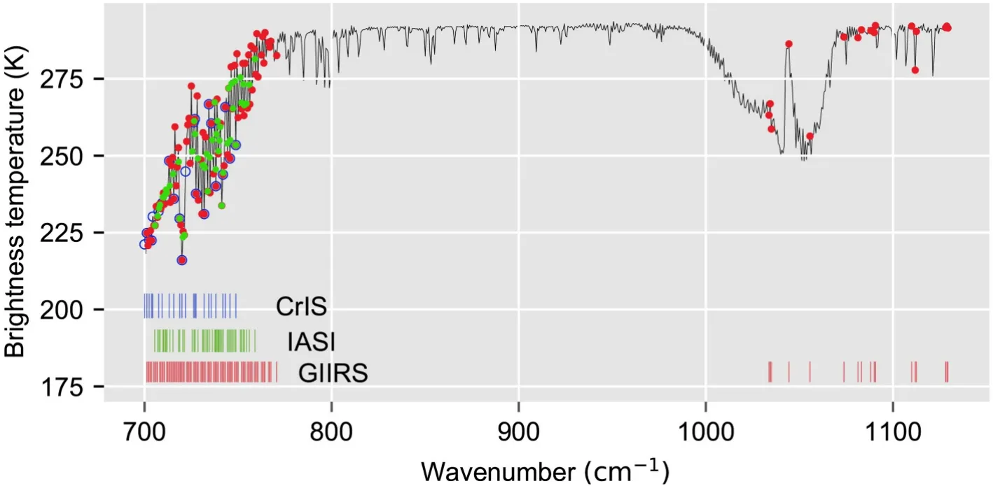
Fig. 8. A comparison of the 23 temperature channels of CrIS, 49 temperature channels of IASI, and 106 temperature channels of GIIRS selected using our method in the longwavelength band (700−1130 cm−1).

Table 3. The GIIRS temperature channel selection at 700−780 cm−1. A total of 89 comparable channels are in the list for retrieval validation. The first column represents the index value of the channel. The second column represents the wave number corresponding to the channel. In the third column, channel markers C0, C1, C2 and C3 indicate which central sequence was selected from.

Table 3. (Continued.)

Fig. 9. Comparison of the retrieval performance of different temperature channel subsets under a different number of hidden layer neurons in the comparable band (700−780 cm−1). From left to right, the number of hidden layer neurons in each row’s subplot is 55, 23, 12 and 10, respectively. The number of input neurons is set to (a−d) 89, corresponding to the number of GIIRS temperature channels; (e−h) 49, corresponding to the number of temperature channels of IASI; and (i−l) 23,corresponding to the number of temperature channels of CrIS.
Instead of using the overall testing set to evaluate the models, we analyzed the retrieval performance at each selected pressure level (Fig. 10). In general, increasing the number of input neurons or neurons in the hidden layer increases the retrieval accuracy at each pressure level. The reason is that a more complex neural network model can achieve better approximations. Specifically, for our temperature retrieval model, more input neurons means that more energy information of the brightness temperature spectrum can be learned, especially using the channel subset selected by the SSA method proposed as the input, when compared with the other two channel subsets. Likewise, more hidden layer units also enhances the learning ability of the model.Thus, the model with 89 input neurons and 55 hidden layer neurons provided the best performance at each pressure level. It should be mentioned that, although the performance of the selected channels has been verified through ANN models, the RMSE values are relatively high compared to community practice due to the limitations of matched samples and model architecture. These issues will be addressed in subsequent studies.
In each model, the retrieval result at 850 hPa is always the most accurate of all the levels. However, changes in model structure do not further significantly improve its accuracy. When the number of hidden layer nodes is 55, our channel subset slightly reduces the values of RMSE and MAE,but significantly improves the performance at pressure levels above 850 hPa, especially at 500 hPa. Wang and Wei(2012) noted that the accuracy of the 500 hPa geopotential height forecast is an important and classical measure of forecast skill.
Even though the accuracy of the temperature retrieval near 825 hPa is high, the R2score at this level is much smaller than that of the other levels, indicating that there is little variation in the temperature values at this pressure level.Hence, a small prediction error will affect the R2score. The R2score at all other pressure levels is higher when using the best model.
6. Conclusions
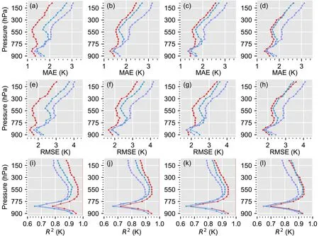
Fig. 10. Comparison of the retrieval performance of different temperature channel subsets at selected pressure levels under different number of neurons in the hidden layer. From left to right, the number of hidden layer neurons in each column of subplots is 55, 23, 12 and 10. In each subplot, the number of channels corresponding to the red, blue, and purple lines is 89,49 and 23, respectively, which is the number of temperature channels of GIIRS, IASI, and CrIS in the comparable range(700−780 cm−1).
In this paper, we have proposed a novel method for temperature channel selection based on SSA for retrieving atmospheric temperature profiles from FY-4A/GIIRS. The method is effective for dimensionality reduction of hyperspectral infrared data, and has the simplicity and rapidity of the PCA method as well as the interpretability of the conventional channel selection method. In the experimental procedure, our method can amplify more detailed energy variation information in the temperature-sensitive band and obtain more channels in GIIRS’s specific detection range. Through validation using neural networks with different architectures, the temperature channel subset of GIIRS selected using our method has a better performance when compared with that of IASI and CrIS selected using different methods.Two useful results were found in the validation stage: the retrieval is more accurate for lower pressure levels than for upper levels; and the best retrieval verification results were obtained using our chosen temperature channels as inputs and the proposed number of hidden layer nodes (55). In particular, the retrieval accuracy at 500 hPa was improved.
Acknowledgements.We would like to thank the National Satellite Meteorological Center for providing the remote sensing data, and the National Meteorological Information Center for providing the radiosonde data. We would like to thank the anonymous reviewers for their insightful comments on this paper.
 Advances in Atmospheric Sciences2020年7期
- Advances in Atmospheric Sciences的其它文章
- Could the Recent Taal Volcano Eruption Trigger an El Niño and Lead to Eurasian Warming?
- Estimation of PM2.5 Mass Concentration from Visibility
- Modeling the Impacts of Nitrogen Dynamics on Regional Terrestrial Carbon and Water Cycles over China with Noah-MP-CN
- Impacts of Urbanization on the Precipitation Characteristics in Guangdong Province, China
- Isentropic Analysis of Regional Cold Events over Northern China
- Evolution of the Mid-tropospheric Vortex during the Formation of Super Typhoon Megi (2010)
